An Improved Image Retrieval System using Image
Classification
Ashish Oberio
Assistant Professor, Department Of Computer Science & Engineering, Maharishi Markendeshwar
University, Mullana, Ambala
Meenal Raheja
Department Of Computer Science & Engineering, Maharishi Markendeshwar University, Mullana,
Ambala
ABSTRACT
An image retrieval system is a computer system for browsing, searching and retrieving image using the actual content of image like visual features of an image as color, texture, shape, rotation, scaling factor and spatial layout. Now a days, retrieval of image from a large database are based on their visual similarity. The proposed Image retrieval system allows automatic extraction of target image according to object feature of the image itself. The proposed system is to improve the performance of image retrieval system using image classification. To improve existing image retrieval system, image decomposition, feature extraction and image matching mechanism should be improved. For image decomposition, modified Haar Wavelet Transform and D4 Wavelet Transform, to decompose color image into multilevel scale and for the conversion of wavelet coefficients has been used. Furthermore, progressive image retrieval strategy to achieve flexible CBIR is incorporated. The image feature are extracted by using Scale Invariant Feature Transform (SIFT). This approach relies on the choice of several parameters which directly impact its effectiveness when applied to retrieve image. Image matching is done by using NNS algorithm in KD-tree. The proposed system has demonstrated a improved image retrieval system on various database include WANG, MirFlickr, CLEF that containing approximately 15,000 color images.
.
General Terms
Image Processing, Pattern Recognition, SIFT Algorithms
Keywords
Image retrieval system, SIFT, Haar Wavelet transform, D4 Wavelet Transform, Feature Extraction, Kd-tree Algorithm.
1.
INTRODUCTION
The main purpose of the classification process is to categorize all pixels in a digital image into one of several classes. An image retrieval system is a computer system for browsing, searching and retrieving image using the actual content of image like visual features of an image as color, texture, shape, rotation, scaling factor and spatial layout. Now a days, retrieval of image from a large database are based on their visual similarity. With the increasing growth of computer technology, rapidly declining cost of storage and ever-increasing access to the Internet, digital acquisition of information has become increasingly popular in recent years. Digital information is preferable to analog formats because of convenient sharing and distribution properties. This trend has
motivated research in image databases, which were nearly ignored by traditional computer systems due to the enormous amount of data necessary to represent images and the difficulty of automatically analyzing images.
Content Based Image Retrieval is to retrieve an image from the image database when given a query image. Query Image is the users target image for the searching process. CBIR systems operate in two phases: indexing and searching. In the indexing phase, each image of the database is represented using a set of image attribute, such as color, shape, texture and layout. Extracted features are stored in a feature database. In the searching phase, when a user makes a query, a feature vector for the query is computed. Using a similarity criterion, this vector is compared to the vectors in the feature database. The images most similar to the query are returned to the user. Rapid advances in hardware technology and growth of computer power make facilities for spread use of World Wide Web. This causes that digital libraries manipulate huge amounts of image data. Due to the limitations of space and time, the images are represented in compressed formats. Therefore, new waves of research efforts are directed to feature extraction in compressed domain.
In this paper, we used D4 and Haar wavelet transforms to decompose color images into multilevel scale and wavelet coefficients, with which we perform image feature extraction and similarity match by means of SIFT and NNS in kd-tree algorithm respectively. We also present a progressive retrieval strategy, which contributes to flexible compromise between the retrieval speed and the recall rate. The retrieval performances are compared with the existing wavelet histogram technique. The efficiency in terms Recall rate and retrieval speed is tested with five types of images and the results reflect the importance of wavelets in CBIR. SIFT along with progressive retrieval strategy improves retrieval performance.
2.
IMAGE DECOMPOSITION WITH
WAVELETS
We used two wavelet approaches for color image decomposition, namely Haar, D4 wavelets. These resulting decomposition coefficients are employed to perform image feature extraction and similarity match by virtue of SIFT Algorithm.
2.1
Haar Wavelet Transform
[image:2.595.51.271.198.328.2]Input
Fig 1: Haar Wavelet Forward Transform
If a data set S0, S1 ….SN-1 contains N elements, there will be N/2 averages and N/2 wavelet coefficient values. The averages are stored in the upper half of the N element array and the coefficients are stored in the lower half as shown in the Figure 2. The averages become the input for the next step in the wavelet calculation, where for iteration i+1, Ni+1 = Ni/2. The recursive iterations continue until a single average and a single coefficient are calculated. This replaces the original data set of N elements with an average, followed by a set of coefficients whose size is an increasing power of two (Ex: 20, 21, 22 ... N/2).
The Haar equations to calculate an average𝒂𝒊and a wavelet coefficient 𝒄𝒊from an odd and even element in the data set are
𝑎
𝑖=
𝑆𝑖+𝑆𝑖+12
,
𝑐
𝑖=
𝑆𝑖−𝑆𝑖+12
1
Forward Haar transform for an eight element signal is shown in the Figure 3. Here signal is multiplied by the forward transform matrix. 𝑎0 𝑎1 𝑎2 𝑎3 𝑐0 𝑐1 𝑐2 𝑐3 𝑎0 𝑎1 𝑎2 𝑎3 𝑐0 𝑐1 𝑐2 𝑐3 = 1 2 12 0 0 0 0 0 0 1
2 −1
2 0 0 0 0 0 0 0 0 1
2 1
2 0 0 0 0 0 0 1
2 −1
2 0 0 0 0 0 0 0 0 1
2 1 2 0 0 0 0 0 0 1
2 −1
2 0 0 0 0 0 0 0 0 1
2 1 2 0 0 0 0 0 0 1
2 −1 2 ° 𝑠0 𝑠1 𝑠2 𝑠3 𝑠4 𝑠5 𝑠6 𝑠7 2
Fig 2: Haar Forward Transform For 8 Element Signal
The arrow represents a split operation that reorders the result so that the average values are in the first half of the vector and the coefficients are in the second half. To complete the forward Haar transform there are two more steps. The next step would multiple the average values 𝒂𝒊by a 4x4 transform matrix, generating two new averages and two new coefficients which would replace the averages in the first step. The last step would multiply these new averages by a 2x2 matrix generating the final average and the final coefficient.
2.2
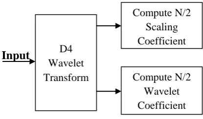
The Daubechies D4 Wavelet Transform
Input
Fig 3: D4 Wavelet Forward Transform
The D4 transform has four wavelet and scaling function coefficients as shown in the Figure 3.The scaling function coefficients are:
0=
1 + 3
4 2
1=
3 + 3
4 2
3
2=
3 − 3
4 2
3=
1 − 3
4 2
4
Each step of the wavelet transform applies the scaling function to the data input. If the original data set has N values, the scaling function will be applied in the wavelet transform step to calculate N/2 smoothed values. In the ordered wavelet transform the smoothed values are stored in the lower half of the N element input vector.
The wavelet function coefficient values are:
𝑔
0=
3; 𝑔
1= −
2; 𝑔
2=
1; 𝑔
3= −
05
Each step of the wavelet transform applies the wavelet function to the input data. If the original data set has N values, the wavelet function will be applied to calculate N/2 differences (reflecting change in the data
Daubechies D4 scaling function
𝑎
𝑖=
0𝑠
2𝑖+
1𝑠
2𝑖+1+
2𝑠
2𝑖+2+
3𝑠
2𝑖+36
[image:2.595.314.522.233.355.2]𝑎 𝑖 =
0𝑠 2𝑖 +
1𝑠 2𝑖 + 1 +
2𝑠 2𝑖 + 2
+
3𝑠 2𝑖 + 3 7
Daubechies D4 wavelet function
𝑐
𝑖= 𝑔
0𝑠
2𝑖+ 𝑔
1𝑠
2𝑖+1+ 𝑔
2𝑠
2𝑖+2+ 𝑔
3𝑠
2𝑖+38
𝑐
𝑖= 𝑔
0𝑠 2𝑖 + 𝑔
1𝑠 2𝑖 + 1 + 𝑔
2𝑠 2𝑖 + 2
+ 𝑔
3𝑠 2𝑖 + 3 9
Each iteration in the wavelet transform step calculates a scaling function value and a wavelet function value.
The index i is incremented by two with each iteration,
and new scaling and wavelet function values are calculated.
D4 forward transform matrix for 8 element signal is shown in the Figure 4.
0 1 2 3 0 0 0 0 𝑔0 𝑔1 𝑔2 𝑔3 0 0 0 0
0 0 0 1 2 3 0 0
0 0 𝑔0 𝑔1 𝑔2 𝑔3 0 0
0 0 0 0 0 1 2 3
0 0 0 0 𝑔1 𝑔2 𝑔3 𝑔4
0 0 0 0 0 0 0 1 2 3
0 0 0 0 0 0 𝑔0 𝑔1 𝑔2 𝑔3
× 𝑠0
𝑠1
𝑠2
𝑠3
𝑠4
𝑠5
𝑠6 𝑠7
[image:3.595.329.544.189.737.2]10
Fig 4: D4 Forward Transform Matrix For 8 Element Signal
3.
PROPOSED IMAGE RETRIEVAL
SYSTEM ARCHITECTURE
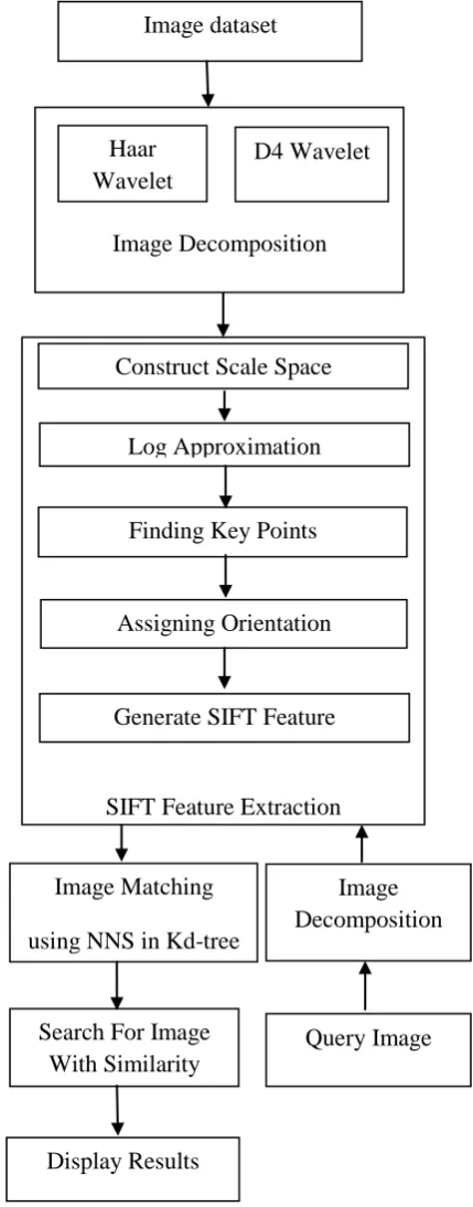
Our proposed IRS algorithm is based on decomposition of the database images using Haar and D4 wavelets in the offline as well as in online for query image. With resulting coefficients using SIFT algorithm we extract the features and perform highly efficient image matching with the help of NNS in Kd-tree algorithm. This done in Various database that contain groups of color images. Fig 5 shows its structure.
Database used are : WANG, MirFlickr, CLEF . In this paper, we used D4 and Haar wavelet transforms to decompose color images into multilevel scale and wavelet coefficients, with which we perform image feature extraction and similarity match by means of SIFT and NNS in kd-tree algorithm respectively. We also present a progressive retrieval strategy, which contributes to flexible compromise between the retrieval speed and the recall rate. The retrieval performances are compared with the existing wavelet histogram technique.
4.
FEATURE EXTRACTION USING
SIFT
Image matching is a fundamental aspect of many problems in computer vision, including Content based image retrieval. For any object in an image, interesting points on the object can be extracted to provide a "feature description" of the object. This description, extracted from a training image, can then be used to identify the object when attempting to locate the object in a test image containing many other objects. To perform reliable recognition, it is important that the features extracted from the training image be detectable even under changes in image scale, noise and illumination. Such points usually lie on high-contrast regions of the image, such as object edges. SIFT
keypoints of objects are first extracted from a set of reference images and stored in a database. An object is recognized in a new image by individually comparing each feature from the new image to this database and finding candidate matching features based on Euclidean distance of their feature vectors. From the full set of matches, subsets of keypoints that agree on the object and its location, scale, and orientation in the new image are identified to filter out good matches.
[image:3.595.53.280.280.381.2]The SIFT algorithm consists of following four major steps :
Fig 5: Proposed Image Retrieval System Architecture
SIFT Feature Extraction
Construct Scale Space
Log Approximation
Finding Key Points
Assigning Orientation
Generate SIFT Feature
Image Matching
using NNS in Kd-tree
Search For Image
With Similarity
Display Results
Query Image
Image
Decomposition
Image dataset
Image Decomposition
Haar
Wavelet
4.1
Scale Space Extrema Detection
The first step in the algorithm is to identify location and scales that can be repeatedly assigned under differing views of the same object. Multiscale image Lx,y,is obtained by
convolving the image I
x, y
with variable scaleGaussian
𝐿 𝑥, 𝑦, 𝜎 = 𝐺 𝑥, 𝑦, 𝜎 ∗ 𝐼 𝑥, 𝑦 11
Where * is the convolution operation in x and y, 𝜎 is scale
co-ordinates and
𝐺 𝑥, 𝑦, 𝜎 =
1 2𝜋𝜎2𝑒
− 𝑥2+𝑦 2 2𝜎 2
For effectively detecting key points locations in scale space, Lowe used scale space extrema in the difference-of- Gaussian
(DoG) function convolved with the image,
D
x
,
y
,
which can be computed from the difference of two nearby scales separated by a constant multiplicative factor k:𝐷 𝑥, 𝑦, 𝑘
1, 𝜎 = 𝐺 𝑥, 𝑦, 𝑘
2, 𝜎 − 𝐺 𝑥, 𝑦, 𝑘
1, 𝜎
∗ I x, y
= 𝐿 𝑥, 𝑦, 𝑘
2, 𝜎 − 𝐿 𝑥, 𝑦, 𝑘
1, 𝜎 12
To detect the local maxima and minima of
D
x
,
y
,
, each sample point is compared to its eight neighbors in the current image and nine neighbors in the scale above and below see figure . It is selected only if it is larger or smaller than all of these neighbors..
4.2
Key Point Localization
This stage attempts to eliminate more points from the list of key points by finding those that have low contrast or are poorly localized on an edge. Once a keypoint has been found by comparing a pixel to its neighbor, the next step is to perform a detailed fit to the nearby data for location, scale and ratio of principle curvatures. This information allows points to be rejected that have low contrast and poorly localized along an edge. The approach use Taylor expansion of the Scale– Space function.𝐷 𝑥, 𝑦, 𝜎 , shifted so that the origin is at the same point.
𝐷 𝑥 = 𝐷 +
𝛿𝐷
𝑇𝛿𝑋
𝑋 +
1
2
𝑋
𝑇𝛿
2𝐷
𝛿𝑋
2𝑋 13
4.3
Orientation Assignment
The dominant orientation is assigned to each keypoint based on local image gradient directions. The gradients magnitude
m(x, y) and orientations (x, y) is computed using pixel differences:
𝑚 𝑥, 𝑦
= 𝐿 𝑥 + 1, 𝑦 − 𝐿 𝑥 − 1, 𝑦 2+ 𝐿 𝑥, 𝑦 + 1 − 𝐿 𝑥, 𝑦 − 1 2 14
𝜃 𝑥, 𝑦
= tan−1 𝐿 𝑥, 𝑦 + 1 − 𝐿 𝑥, 𝑦 − 1
𝐿 𝑥 + 1, 𝑦 − 𝐿 𝑥 − 1, 𝑦 15
Dominant orientation is determined by building a histogram of gradient orientations from the neighborhood of keypoints. The highest peak in the histogram is detected, and then any other local peak that is within 80% of the highest peak is used to also create a keypoint with that orientation.
4.4
Key Point Descriptors
For each keypoint, the keypoint descriptor is created by sampling the magnitudes and orientations of the image gradients in the N ×N neighboring region around the point.
5.
IMAGE MATCHING
Image matching is done using NNS (nearest neighbor search ) algorithm in a kd-Tree. However, though the matching utilizes a NNS, the criterion for a match is not to be a nearest neighbor; then all nodes would have a match. The comparison is done from the source image, to the compared image. Thus, in the following outline, to “select a node” means to select a node from the keypoints of the source image.
The Algorithm follows as:
Step 1: Select a node from the set of all nodes not yet selected.
Step 2: Mark the node as selected.
Step 3: Locate the two nearest neighbors of the selected node.
Step 4: If the distances between the two neighbors are less than or equal to a given distance, we have a match. Mark the keypoints as match
Step 5: Perform step 1-4 for all nodes in the source image.
The key step of the matching algorithm is step 4. It is here it is decided whether the source node (or keypoint) has a match in the compared set of keypoints, or not. The image matching algorithm verifies the distance between the two closest neighbors of a source node. If the distance is within a given boundary, the source node is marked as a match.
5.1
Feature Vector And Similarity Criteria
The feature vector of each image is defined at different levels. At Lth level and ith leaf nodes, feature vector Li F is given as𝐹
𝐿𝑖= 𝑚
𝑖𝑤
𝑖16
𝑤
𝑖= ln
N
N
i17
where mi –number of descriptor vectors of database image pass through the leaf node i
wi – weight of leaf node i,
N – Total number of images in the database
Ni – Number of images in the database with at least one
descriptor vector pass through node i.
Similarly, normalization is used to achieve the fairness between database images with different descriptor vectors. Therefore, the normalized feature vectors at level L and node i
is
𝐹
𝑛𝑜𝑟=
F
LiIn the proposed method, a scoring is used as a similarity easure which calculate the score between query 𝑄𝑖and database image as 𝐼𝑖 given in following equation.
𝑆𝑐𝑜𝑟𝑒 = 𝐹
𝑄𝑖× 𝐹
𝐼𝑖𝑃
𝑖=0
19
Where
𝐹
𝑄𝑖- Feature vector of query image ;P
-Number of leaf nodes;𝐹
𝐼𝑖 - Feature vector of image in the database. Highest scoring database image is considered as more relevant image to query one.5.2
Feature Extraction And Image
Matching Follow These Steps
Step1: The algorithm SIFT first computes the a descriptor for each query image in the database. Constructing a scale space is the initial preparation. Internal representations of the original image are created to ensure scale invariance. Step2: SIFT computes the descriptor for each query image in the database. Unwanted keypoints like edges and low contrast regions are eliminated by DOG.
Step3: An orientation is calculated for each key point. Any further calculations are done relative to this orientation, making it rotation invariant.
Step4: SIFT matches the key points of query image with the key points of each of the query results of the Image Retrieval System using NNS. They are then ranked as per number of matching key points.
6.
EXPERIMENTATION RESULT
The general flow of the experiments starts with the decomposition of data base image using Haar and D4 wavelet in offline. The maximal decomposition level J = 4. With SIFT we extracted the image feature vector and performed highly efficient image matching. We used progressive retrieval strategy to balance between computational complexity and retrieval accuracy. Focuses on the comparison of two important retrieval indices, namely retrieval accuracy and the speed. The test image database contains over 15,000 images of 24 bits true color. They are divided into 3 Dataset Wang, Mirflickr and clef. These Three groups containing realistic images worldwide. For simplicity, all images are pre processed to be 256x256 sizes before decomposition. The Recall rate is defined as the ratio of the number of relevant (same category) retrieved images to the number of relevant items in collection.
𝑅𝑒𝑐𝑎𝑙𝑙 𝑅𝑎𝑡𝑒 = 𝑁𝑢𝑚𝑏𝑒𝑟 𝑜𝑓 𝑟𝑒𝑙𝑒𝑣𝑎𝑛𝑡 𝑟𝑒𝑡𝑟𝑖𝑒𝑣𝑒𝑑 𝑖𝑚𝑎𝑔𝑒𝑠 𝑁𝑢𝑚𝑏𝑒𝑟 𝑜𝑓 𝑟𝑒𝑙𝑒𝑣𝑎𝑛𝑡 𝑖𝑡𝑒𝑚𝑠 𝑖𝑛 𝑐𝑜𝑙𝑙𝑒𝑐𝑡𝑖𝑜𝑛
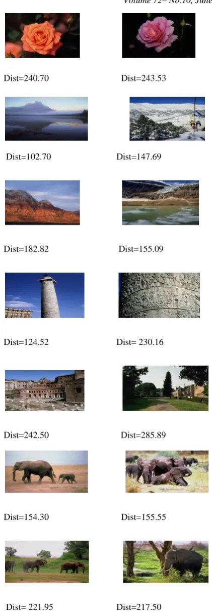
WANG DATABASE
Dist=182.60 Dist=211.97
Dist=240.70 Dist=243.53
Dist=102.70 Dist=147.69
Dist=182.82 Dist=155.09
Dist=124.52 Dist= 230.16
Dist=242.50 Dist=285.89
Dist=154.30 Dist=155.55
Dist= 221.95 Dist=217.50
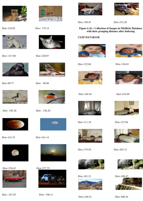
[image:5.595.312.523.59.669.2]MIRFLICKR DATABASE
Dist=154.82 Dist= 179.14
Dist =217.00 Dist=228.97
Dist=90.77 Dist= 98.88
Dist= 185.26 Dist= 236.20
Dist=141.53 Dist=161.14
Dist=258.42 Dist=277.75
Dist= 167.29 Dist= 190.11
Dist=198.45 Dist=233.20
Figure 6 (b) : Collection of Images in Mirflickr Database with their grouping distance after Indexing
CLEF DATABASE
Dist=125.86 Dist=126.83
Dist=169.36 Dist=234.50
Dist=111.18 Dist=127.04
Dist=179.58 Dist=203.12
Dist=181.31 Dist=189.47
[image:6.595.47.540.81.774.2]
Dist=148.09 Dist=162.29
Dist=173.09 Dist=254.18
Fig 6 (c) : Collection of Images in Clef Database with their grouping distance after Indexing
Figure 6 (a), (b), (c) shows the three different dataset images in which testing of this image retrieval system is done. In above figures, categories of images are different from each other. Calculate their precision value with precise threshold 0.5 and rough filtering threshold 0.3. Wang dataset contains about 10,000 images, Mirflickr Dataset contain around 5000 images and Clef Dataset contain 2400 images.
Table 1 shows the comparison between each dataset using precision value and recall rate. Focuses on the comparison of two important retrieval indices, namely retrieval accuracy and the speed.
Table 1: Comparison Of Precision value and Recall Rate for Various Dataset Used In This System
Databases
Average
Precision
Recall Rate
(%age)
WANG
Database
0.89
92%
MirFlickr
Database
0.83
81%
CLEF
[image:7.595.315.560.66.290.2]Database
0.73
88%
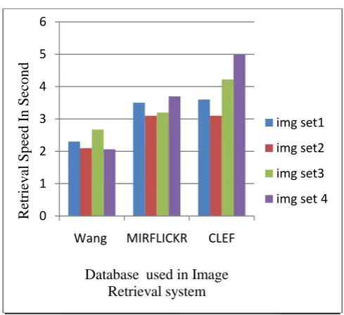
Fig 7 : Analysis of speed on different dataset using NNS in kd-tree
Figure 7 show the time to retrieve an image from dataset by using NNS in kd-tree where img set1, img set2 ,img set3, img set4 is the image set from wang, mirflickr, Clef dataset respectively as shown in figure 6 (a), (b), (c). The result shows accurate retrieval system as time to retrieve an image is comparatively less from retrieve image without using NNS in kd-tree as shown in figure 8.
Fig 8 : Analysis of speed on different dataset without using NNS in kd-tree
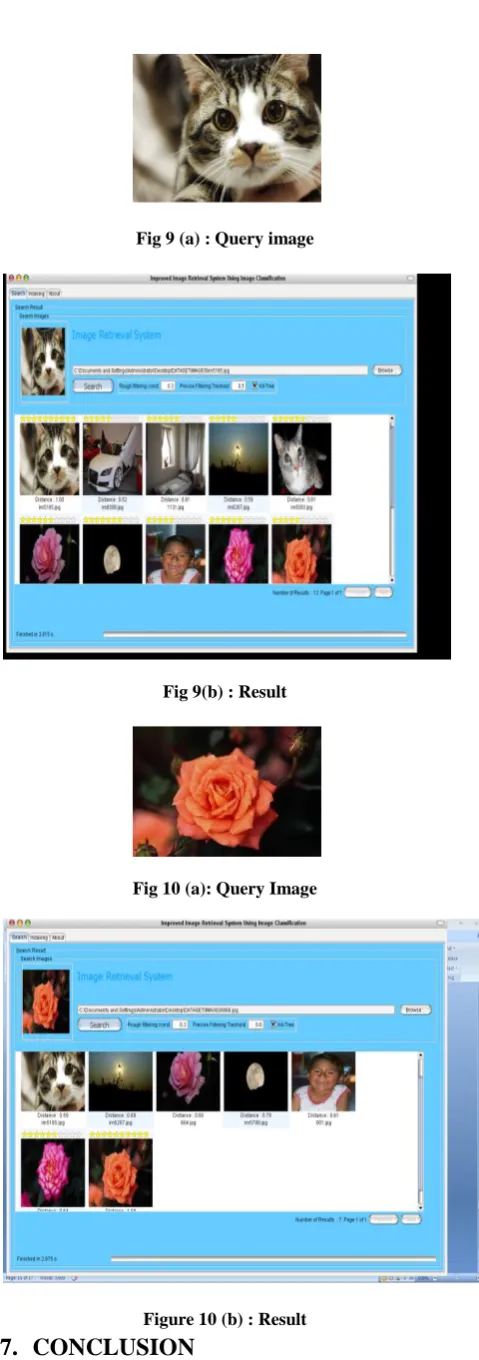
Image Query and Results
The following are the query and search results produced by the program. Fig. 9(a), Fig. 10 (a) and Fig. 11 (a) are query images and Fig. 9 (b), Fig. 10 (b), Fig. 11 (b) are their respective top results.
0 1 2 3 4 5 6
Wang MIRFLICKR CLEF
img set1
img set2
img set3
img set 4
R
et
ri
ev
al
Speed
In
Second
Database used in Image
Retrieval system
0 1 2 3 4 5 6 7 8
Wang MIRFLICKR CLEF
img set1
img set2
img set3
img set 4
R
et
ri
ev
al
Speed
In
Second
[image:7.595.54.278.85.298.2] [image:7.595.316.566.425.646.2] [image:7.595.50.290.492.696.2]Fig 9 (a) : Query image
Fig 9(b) : Result
Fig 10 (a): Query Image
Figure 10 (b) : Result
7.
CONCLUSION
The primary aim of the thesis to implement an image retrieval system was successfully accomplished and its performance was also, measured and analyzed. The proposed system test
on three different database and WANG Database gives faster result in terms of speed and accuracy. In addition, the progressive retrieval strategy helps to achieve flexible compromise among retrieval results. We conclude from the results that wavelets achieve high retrieval performance in real time systems. SIFT could be an extremely robust resource for object detection and image matching. SIFT calculates the key points of query just once and uses number of matching key points with the query image to rank them. We use the location, scale and orientation of the images to match key-points of the query image and the images returned by Image retrieval system. We have thus utilized the best features of both the algorithms to speed up the search and improve the accuracy.
8.
REFERENCES
[1] Y. Rui, T.S. Huang, M. Ortega, S. Mehrotra, 1998. “Relevance feedback: a power tool for interactive content-based image retrieval,” IEEE Trans. Circuits Systems Video Technol. 8 (5), pp. 644–655
[2] J.Z. Wang, J. Li, G. Wiederhold, and O. Firschein, 1998,ªSystem for Screening Objectionable Images, “ Computer Comm.”, vol. 21, no. 15, pp. 1355-1360 [3] A. W. M. Smeulders, M. Worring, S. Santini, A. Gupta,
and R. Jain,“Content-based image retrieval at the end of the early years,” IEEETrans. Dec.2000 Pattern Anal. Mach. Intell., vol. 22, no. 12, pp. 1349–1380,.
[4] James Z. Wang, Jia Li , SEPTEMBER2001 ,“SIMPLICITY: Semantics-Sensitive Integrated Matching for Picture Libraries”, IEEE TRANSACTIONS ON PATTERN ANALYSIS AND MACHINE INTELLIGENCE, VOL. 23, NO. 9, [5] K. Mikolajczyk, C. Schmid, “A performance evaluation
of local descriptors,” In: Proc. IEEE Conf. on Computer Vision and Pattern Recognition (CVPR), pp. 257– 264, 2003.
[6] K. Mikolajczyk, T. Tuytelaars, C. Schmid, A. Zisserman, J. Matas, F. Schaffalitzky, T. Kadir, L.V. Gool, 2005 , “A comparison of affine region detectors,” Int. J. Comput. Vision vol. 65 , no. (1/2), pp. 43–76 [7] D. Nister and H. Stewenius. Scalable recognition with a
kd-tree . 2006, In Proc. IEEE Conference on Computer Vision and Pattern Recognition, volume 2, pp. 2161 – 2168.
[8] D. Nister and H. Stewenius, “Scalable Recognition with a Vocabulary Tree,2007,” IEEE Computer Society Conference on Computer Vision and Pattern Recognition, pp.2161-2168, 2006. Y. Liu, D. Zhang, G. Lu, W. Y. Ma, “A survey of content-based image retrieval with high-level semantics, “Pattern Recognition, vol. 40, pp. 262-282.
[9] Z. Wang, K. Jia, P. Liu, “A Novel Image Retrieval Algorithm Based on ROI by using SIFT Feature Matching,” International Conference on MultiMedia and Information Technology, IEEE Computer Society, Washington DC, pp.338-341,2008.
[10]Deslaers, T., Keysers, D., Ney, H.: Features for image retrieval: an experimental comparison. Information Retrieval, vol. 11, 77–107. 2008
[image:8.595.54.294.45.726.2]