Munich Personal RePEc Archive
Incorporating spatial variation in housing
attribute prices: A comparison of
geographically weighted regression and
the spatial expansion method
Bitter, Chris and Mulligan, Gordon and Dall’erba, Sandy
2006
Online at
https://mpra.ub.uni-muenchen.de/1379/
Incorporating spatial variation in housing attribute prices: A
comparison of geographically weighted regression and the spatial
expansion method
Christopher Bitter, Gordon F. Mulligan, and Sandy Dall’erba
The University of Arizona
Department of Geography and Regional Development Harvill Building Box #2
Tucson, Arizona
Abstract
Hedonic house price models typically impose a constant price structure on housing characteristics throughout an entire market area. However, there is increasing evidence that the marginal prices of many important attributes vary over space, especially within large markets. In this paper, we compare two approaches to examine spatial heterogeneity in housing attribute prices within the Tucson, Arizona housing market: the spatial
expansion method and geographically weighted regression (GWR). Our results provide strong evidence that the marginal price of key housing characteristics varies over space.
GWR outperforms the spatial expansion method in terms of explanatory power and predictive accuracy.
Key words: hedonic model, house price, spatial heterogeneity, expansion method, geographically weighted regression
JEL classification: C31, C51, C52, R21, R31
1 Introduction
The importance of location in determining housing prices is widely recognized.
Controlling for location and the spatial structure of markets is thus essential to explaining house price differentials and deriving accurate coefficient estimates in hedonic house price models. However, spatial issues have not always been given adequate attention in hedonic applications (Bowen et al. 2001, Páez et al. 2001). Key econometric issues include spatial dependence and spatial heterogeneity (Anselin 1988; 1990). While housing markets are likely to be characterized by both, we focus specifically on the issue of spatial heterogeneity as it has received less attention in the literature.
Within the housing market context, the issue of spatial heterogeneity centers on whether the marginal price of housing attributes is constant throughout a metropolitan area or vary over space. Most empirical models have conceptualized a metropolitan area as a single unified market, and while neighborhood effects may be incorporated into regression models through varying intercepts, the coefficients of structural attributes are held
constant throughout the market (Ordford 1999). If spatial heterogeneity exists, stationary coefficient models will produce parameters that are in essence an “average” value of the parameter over all locations. A failure to incorporate spatial heterogeneity will result in biased coefficients and a loss of explanatory power and may obscure important dynamics relating to the operation of housing markets.
This paper seeks to add to our understanding of the role that spatial heterogeneity plays in housing markets by comparing two methods that allow spatially varying parameters in an analysis of the Tucson, Arizona housing market. The spatial expansion method,
pioneered by Casetti (1972), allows parameters to vary over space in a traditional OLS regression framework by interacting house characteristics with locational information. Geographically weighted regression in essence specifies a separate regression model at every observation point, thus enabling unique coefficients to be estimated at each location (Brunsdon et al. 1996).
The remainder of the paper is organized as follows. We begin with a review of the pertinent literature followed by an overview of the Tucson housing market. Next, the data and methodology employed in the study are detailed. We then compare the results of the models and discuss the spatial patterns observed in the data. In the final section we draw conclusions and suggest avenues for future research.
2 Spatial variation in housing attribute prices
There is good reason to expect that the price of housing attributes will exhibit spatial heterogeneity within large housing markets due to localized supply and demand
metropolitan area homes tend to be older and frequently lack features such as large garages, when compared to those located at the suburban fringe. Housing is a unique good due to its fixed location and durability, and the characteristics of the housing stock may be difficult to change in response to changing demand. Thus the supply of certain types of housing and neighborhood characteristics may be highly inelastic, particularly over short periods of time (Schare and Struyk 1975).
Demand by households for specific structural and locational attributes is known to vary based on socioeconomic status, household status, race and ethnicity (Quigley 1985), as well as the location of household activities such as the workplace. Demand for some attributes, such as a high quality school district or for a house with a minimum number of bedrooms, may also be highly inelastic (Schare and Struyk 1975). Thus all housing within a large metropolitan area will not be substitutable. In addition, access to information and the actions of market participants such as realtors, lenders, and
appraisers may constrain households from participating in all segments of a large market (Michaels and Smith 1990).
Changes in household preferences for housing characteristics and locational attributes, as well as the characteristics of neighborhoods themselves, may result in spatial mismatches between supply and demand as the housing stock available within a particular geographic area may not match current demand. Greater competition for those housing attributes that are in high demand, yet locally scarce, should result in higher marginal prices. Thus one would expect supply and demand imbalances to result in spatial heterogeneity within large housing markets.
One approach to dealing with spatial heterogeneity is to delineate the housing market into distinct geographic areas or submarkets and to estimate separate hedonic prices schedules for each (Schnare and Struyk, 1975, Goodman 1981; 1998, Michaels and Smith 1990, Bourassa et al. 2003). However, housing submarkets are often problematic to define in practice and this approach makes it difficult to generalize about the dynamics of the broader housing market or urban area. The focus on housing submarkets also posits that spatial heterogeneity is a discrete phenomenon and does not allow attribute prices to vary in a continuous manner over space.
A number of housing market studies have used variants of the expansion method pioneered by Casetti (1972). This method recognizes that functional relationships may not be constant but vary over space, and explicitly allows parameter estimates to “drift” based on their spatial context (Jones and Casetti 1992). This method is operationalized by “expanding” the parameters of stationary coefficient models.
for neighborhoods with similar “quality” scores regardless of the supply of specific housing characteristics in each. Theriault et al. (2003) improves upon this approach with an expansion model that allows housing attributes to vary based on both accessibility and neighborhood attributes.
In a study of Tucson, Arizona, Fik, Ling, and Mulligan (2003) specified a “fully
interactive” expansion model employing a second order polynomial expansion of housing attributes, the properties’{x, y} coordinates, and dummy variables representing
submarkets. The interactions between the absolute location variables and structural attributes thus allowed the coefficients to vary over space. This model outperformed stationary model specifications and its explanatory power was far superior. A number of the spatial interactive terms were significant, indicating the presence of spatial
heterogeneity in the prices of these attributes. A limitation of this study is that it relied on only three housing attribute variables, thus making it difficult to assess whether observed price variation was the result of intrinsic parameter variation or due to the effects of omitted variables.
Incorporating absolute location into hedonic models in the form of a polynomial expansion of parcel coordinates1 is appealing because it is difficult if not impossible to identify and accurately specify all locational influences that affect housing prices (Ordford 1999). While a parcel’s coordinates are not a direct determinant of housing prices, they may serve a useful role in controlling for the influence of location on prices. A number of other authors have experimented with this approach in recent years (Clapp 2001, Pavlov 2000).
Geographically Weighted Regression (GWR) is a local modeling approach that explicitly allows parameter estimates to vary over space (Brunsdon et al. 1996). Rather than specifying a single model to characterize the entire housing market, GWR estimates a separate model for each sale point and weights observations by their distance to this point, thus allowing unique marginal-price estimates at each location. This method is appealing because it mimics to some extent the “sales comparison” approach to valuation used by appraisers in that only sales within close proximity to the subject property are considered, and price adjustments are made based on differences in characteristics within this subset of properties.
GWR has not been widely utilized in the housing market context. The only application the authors are aware of is a recent study of the Toronto, Canada housing market by Farber and Yeats (2006). In this study, GWR outperformed several alternative
approaches and was able to explain more than 90% of the variation in housing prices and provided evidence for spatial heterogeneity in several housing attributes. Páez (2005) compares GWR and the expansion method in a simulation study, finding that both approaches are able to provide a reasonable representation of the spatial patterns inherent in the simulated data. However, no studies have provided a direct comparison between the two methods in the analysis of house prices.
1
3 Tucson housing market
Tucson is a mid-sized metropolitan area situated within the Sonoran Desert in Southern Arizona and is ringed by mountain ranges. Like many western cities, much of the land surrounding the urbanized area is publicly owned. The City of Tucson has been one of the nation’s fastest growing cities over the past several decades, with its population expanding from 330,000 in 1980 to 487,000 in 2000, while the greater metropolitan area (Pima County) saw its population swell from 530,000 to 850,000 during the same period. The population is diverse, with Hispanics accounting for nearly 30% of the total
population (Mulligan et al. 2000).
Like most southwestern cities, Tucson’s development pattern is relatively dispersed and the urbanized area encompasses some 500 square miles. The metro’s transportation system is designed largely for private automobiles. While some central neighborhoods are densely populated, most residents live in suburban style settings. Tucson’s
employment too, is dispersed with its weak CBD functioning primarily as a government services center. Large area employers include The University of Arizona,
Davis-Monthan Air Force Base, and Raytheon.
Tucson’s housing market is generally differentiated from north to south, with the highest priced housing found in the foothills of the Santa Catalina Mountains located to the northeast of Central Tucson (see Figure 1). The northern half of the city typically contains newer, larger, more expensive housing units than those found in the southern and central areas, although new development is occurring at the urban fringe in all directions. The eastern and western portions of the market generally exhibit “average” house characteristics.
Following a prolonged slump during the early 1990s, the Tucson housing market was generally stable during the mid 1990s. By the end of the decade prices began to appreciate again in real terms. During recent years house price appreciation has accelerated rapidly with price increases of 13.4% and 30.6% in 2004 and 2005 respectively (National Association of Realtors, 2006).
4 Data and methods
4.1 Data
Figure 1. Study Area
The analytical database was constructed as follows: We first selected sales records representing detached single-family homes. These sales were then matched to a separate assessment “structural file” containing information on the characteristics of each
dwelling. Next, these data were matched to a property “parcel” GIS coverage maintained by Pima County and each property was attributed with the coordinates of its parcel centroid. This resulted in a total of 14,154 matched records. A large number of records were missing lot sizes in the structural file, as the assessor no longer routinely tracks this information. In these cases we attributed the records with the area of the property’s parcel polygon from the GIS coverage2.
We then selected a subset of records corresponding to the contiguous Tucson urbanized area, as much of the county is rural. Our data includes all or portions of the
municipalities of Tucson, South Tucson, Marana, and Oro Valley, as well as portions of unincorporated Pima County. Records that did not represent “arms length” transactions, were missing data elements, or were outliers in terms of price or structural attributes were also eliminated. Our final data set consists of 11,732 records, which represents the vast majority of valid single-family home sales recorded during the year 2000.
4.2 Models
Four models are estimated in the empirical analysis using 90% of the sales, or 10,569 observations. A random sample of 1,163 sales was generated and held out in order to test the predictive accuracy of the various approaches. All models use the natural log of sale price as the dependent variable. While there is no consensus in the literature regarding the appropriate functional form of hedonic house price models (Freeman 2003),
experimentation with the Tucson housing data revealed that the semi-log form performed well in comparison to other common functional forms. Thus the coefficients can be interpreted as the percentage change in sale price attributable to a unit change in an independent variable.
Preliminary regressions established 13 property characteristics to be significant
determinants of housing prices in Tucson. All variables, with the exception of LOTSIZE, as noted above, were taken directly from the assessor’s structural file. Variable
descriptions are provided in Table 1.
We chose to reduce the number of variables entering our models through a principal components analysis because GWR is computationally intensive and the expansion method becomes intractable with a large number of explanatory variables. This is preferred to simply discarding variables as we wish to mitigate the potential for bias resulting from omitted variables. Five variables enter the models individually: SQFT,
2
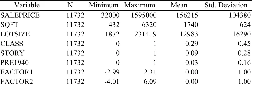
LOTSIZE, STORY, PRE1940, and CLASS. The remaining eight were reduced to two factors. Thus a total of seven variables are used to represent property characteristics (Table 2). Factor one represents newer dwellings with modern features like enclosed garages and refrigerated air conditioning. Factor two represents homes with outdoor amenities such as pools or patios and a high average room size. Full details of the factor analysis are provided in Appendix 1. Correlations between the seven independent variables are relatively low, as only corr (CLASS, SQFT) and corr (FACTOR2, SQFT) exceed 0.5.
Table 1. Independent Variable Descriptions Variable Description
SALEPRICE Selling price in dollars PATIO Number of patios
SQFT Dwelling area in square feet LOTSIZE Size of lot in square feet
ACREF Dummy variable indicating the prescence of regrigerated air conditioning POOLD Dummy variable indicating the presence of a swimming pool
ROOMSF Total number of rooms divided by dwelling size
CLASS Dummy variable indicating high structural quality of the dwelling AGE Age of the dwelling in years
STORY Dummy variable indicating a dwelling of two or more stories BATHROOM Bathroom fixtures divided by the total number of rooms
PRE1940 Dummy variable indicating that the house was built prior to 1940 QUALITY Dummy variable indicating high interior quality of the dwelling GARAGE Dummy variable indicating the presence of a garage on the property
Homes are assigned to a quality and class category by the assessor. The CLASS and QUALITY dummy variables were created by aggregrating the top three and top two categories respectively.
Table 2. Descriptive Statistics
Variable N Minimum Maximum Mean Std. Deviation SALEPRICE 11732 32000 1595000 156215 104380
SQFT 11732 432 6320 1740 624
LOTSIZE 11732 1872 231419 12983 16290
CLASS 11732 0 1 0.29 0.45
STORY 11732 0 1 0.09 0.28
PRE1940 11732 0 1 0.03 0.16
FACTOR1 11732 -2.99 2.31 0.00 1.00 FACTOR2 11732 -4.01 6.09 0.00 1.00
Table 2, as well as nine variables representing absolute location in the form of a third degree polynomial expansion of the parcel coordinates. The raw coordinates were first transformed to deviations from the mean x and y values of all sales within the study area.
Model 2 is the spatial expansion. The seven housing attribute variables are interacted with the nine absolute location variables, thus allowing the marginal price of the housing attributes to vary over space. This results in 63 new independent variables3, in addition to the 16 included in Model 1.
While spatial dependence is not the focus of this paper, we include a spatially lagged dependent variable in Model 3 in order to mitigate potential bias resulting from the omission of this variable. The lag term is calculated as the distance weighted average price of each observation’s 15 nearest neighbors. Although maximum likelihood
estimators have more desirable properties in the presence of spatial dependence, OLS has been employed under certain circumstances involving large data sets (Can and
Megbolugbe 1997; Farber and Yeats, 2006). We follow this approach here. Thus the only difference between Model 2 and Model 3 is the inclusion of the spatial lag term.
Model 4 is the geographically weighted regression model, which was estimated using the GWR 3.0 software package. This model includes the same seven housing attributes as independent variables that were used in the prior models.
As outlined in Fotheringham et al. (2000), the standard hedonic model formulation specifies sale price as a function of a set of housing characteristics as follows:
i k
k ik
i x
y =α0+
∑
α +ε (1)where Xik represents the ith observation of the kth independent variable. The GWR specification is similar, except that unique coefficients are estimated at each observation point: i ik i i k
k u v x
yi =α0 +
∑
α ( , ) +ε (2)where αk(ui,vi) represents the regression coefficient for variable k at regression point i. In matrix notation, the parameters of a GWR model are estimated as follows:
y v u W X X v u W X v
ui, i) ( T ( i, i) ) T ( i, i)
( = −1
α (3)
3
Where W(ui,vi) is a spatial weighting matrix. We utilize a Gaussian function where d represents the Euclidian distance between the regression point and observation point, and h represents the bandwidth as follows:
Wi(ui,vi)=exp(−d/h)2 (4)
The results of GWR are sensitive to the choice of bandwidth, as weighting procedures that specify a wide bandwidth and allow for only minimal distance decay will produce results that are similar to a global model. Conversely, if the bandwidth is narrow only points in close proximity will be considered, which will lead to high variances in the estimators (Fotheringham et al. 2000).
We chose to use an adaptive spatial kernel that allows the bandwidth to vary based on the density of home sales around each regression point, thus encapsulating a smaller area where data is rich and a larger area where data is sparse. This ensures that an equal number of observations will receive a non-zero weighting at all regression points. The cross-validation method, which optimizes the choice through an iterative process based on a least squares criterion, was used to select the bandwidth. The resulting bandwidth is 544 observations.
5 Results
5.1 Model summaries
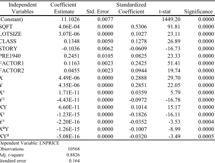
The results for Model 1, in which the marginal-price estimates are held constant throughout the study area, are depicted in Table 3. The global model, utilizing {x , y} coordinates to control for location, does a reasonable job of explaining variation in Tucson house prices as indicated by an adjusted R-squared of 0.88 and standard error of 0.164. All variables are significant at the 0.01 level, have the expected signs, and are of plausible magnitudes.
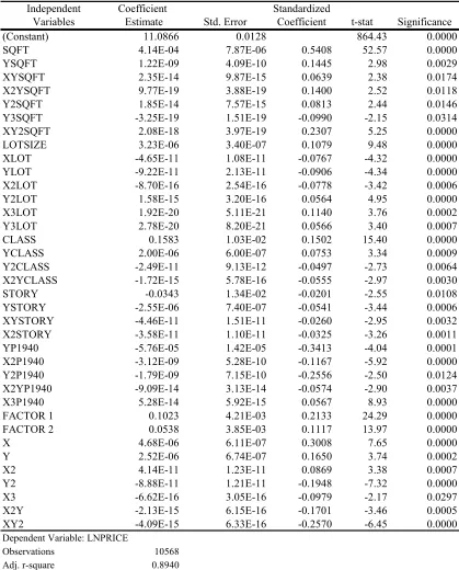
The results for Model 2, the spatial expansion, are shown in Table 4. We report only coefficients that are significant at the 0.05 level, excluding interaction terms involving the two factors. The addition of location-attribute interaction terms results in a modest
Table 3. Model 1 Results: Global
Independent Coefficient Standardized
Variables Estimate Std. Error Coefficient t-stat Significance (Constant) 11.1026 0.0077 1449.20 0.0000 SQFT 4.06E-04 0.0000 0.5306 91.81 0.0000 LOTSIZE 3.07E-06 0.0000 0.1027 23.11 0.0000 CLASS 0.1348 0.0050 0.1278 26.89 0.0000 STORY -0.1036 0.0062 -0.0609 -16.73 0.0000 PRE1940 0.2451 0.0105 0.0825 23.33 0.0000 FACTOR1 0.1163 0.0023 0.2425 51.41 0.0000 FACTOR2 0.0455 0.0023 0.0944 19.74 0.0000 X 4.49E-06 0.0000 0.2888 29.70 0.0000 Y 4.35E-06 0.0000 0.2851 22.05 0.0000 X² 1.71E-11 0.0000 0.0359 5.79 0.0000 Y² -4.43E-11 0.0000 -0.0972 -16.78 0.0000 XY 6.60E-11 0.0000 0.1014 15.17 0.0000 X³ -1.23E-15 0.0000 -0.1826 -16.11 0.0000 Y³ -2.20E-16 0.0000 -0.0352 -3.53 0.0004 X²Y -1.26E-15 0.0000 -0.1007 -8.99 0.0000 XY² -5.08E-16 0.0000 -0.0320 -3.49 0.0005
Dependent Variable: LNPRICE
Observations 10568
Adj. r-square 0.8826
Standard error 0.164
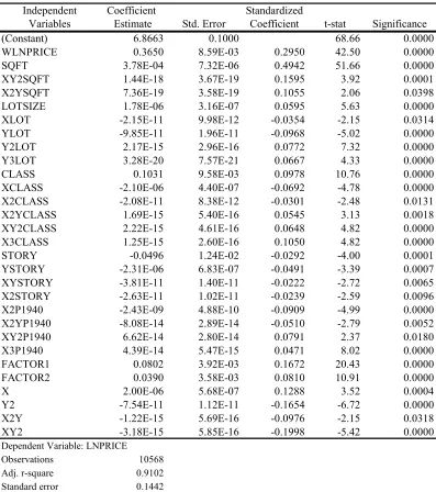
The addition of the spatial lag term in Model 3 results in an improvement in explanatory power as the adjusted R-squared increases from 0.894 to 0.91, while the standard error declines from 0.156 to 0.144 (Table 5). The spatial lag term is positive and significant, suggesting that housing prices are strongly influenced by the prices of nearby homes, or alternatively, features or externalities that homes in close proximity share have not been accounted for in our model. The estimates and significance levels of the housing attributes and location variables generally decline in comparison to Model 2. For example, several of the location variables become insignificant and the marginal-price estimate for LOTSIZE declines markedly.
Table 4. Model 2 Results: Spatial Expansion
Independent Coefficient Standardized
Variables Estimate Std. Error Coefficient t-stat Significance
(Constant) 11.0866 0.0128 864.43 0.0000
SQFT 4.14E-04 7.87E-06 0.5408 52.57 0.0000
YSQFT 1.22E-09 4.09E-10 0.1445 2.98 0.0029
XYSQFT 2.35E-14 9.87E-15 0.0639 2.38 0.0174
X2YSQFT 9.77E-19 3.88E-19 0.1400 2.52 0.0118
Y2SQFT 1.85E-14 7.57E-15 0.0813 2.44 0.0146
Y3SQFT -3.25E-19 1.51E-19 -0.0990 -2.15 0.0314
XY2SQFT 2.08E-18 3.97E-19 0.2307 5.25 0.0000
LOTSIZE 3.23E-06 3.40E-07 0.1079 9.48 0.0000
XLOT -4.65E-11 1.08E-11 -0.0767 -4.32 0.0000
YLOT -9.22E-11 2.13E-11 -0.0906 -4.34 0.0000
X2LOT -8.70E-16 2.54E-16 -0.0778 -3.42 0.0006
Y2LOT 1.58E-15 3.20E-16 0.0564 4.95 0.0000
X3LOT 1.92E-20 5.11E-21 0.1140 3.76 0.0002
Y3LOT 2.78E-20 8.20E-21 0.0566 3.40 0.0007
CLASS 0.1583 1.03E-02 0.1502 15.40 0.0000
YCLASS 2.00E-06 6.00E-07 0.0753 3.34 0.0009
Y2CLASS -2.49E-11 9.13E-12 -0.0497 -2.73 0.0064
X2YCLASS -1.72E-15 5.78E-16 -0.0555 -2.97 0.0030
STORY -0.0343 1.34E-02 -0.0201 -2.55 0.0108
YSTORY -2.55E-06 7.40E-07 -0.0541 -3.44 0.0006
XYSTORY -4.46E-11 1.51E-11 -0.0260 -2.95 0.0032
X2STORY -3.58E-11 1.10E-11 -0.0325 -3.26 0.0011
YP1940 -5.76E-05 1.42E-05 -0.3413 -4.04 0.0001
X2P1940 -3.12E-09 5.28E-10 -0.1167 -5.92 0.0000
Y2P1940 -1.79E-09 7.15E-10 -0.2556 -2.50 0.0124
X2YP1940 -9.09E-14 3.13E-14 -0.0574 -2.90 0.0037
X3P1940 5.28E-14 5.92E-15 0.0567 8.93 0.0000
FACTOR 1 0.1023 4.21E-03 0.2133 24.29 0.0000
FACTOR 2 0.0538 3.85E-03 0.1117 13.97 0.0000
X 4.68E-06 6.11E-07 0.3008 7.65 0.0000
Y 2.52E-06 6.74E-07 0.1650 3.74 0.0002
X2 4.14E-11 1.23E-11 0.0869 3.38 0.0007
Y2 -8.88E-11 1.21E-11 -0.1948 -7.32 0.0000
X3 -6.62E-16 3.05E-16 -0.0979 -2.17 0.0297
X2Y -2.13E-15 6.15E-16 -0.1701 -3.46 0.0005
XY2 -4.09E-15 6.33E-16 -0.2570 -6.45 0.0000
Dependent Variable: LNPRICE
Observations 10568
Adj. r-square 0.8940
Table 5. Model 3 Results: Spatial Expansion with spatial lag term
Independent Coefficient Standardized
Variables Estimate Std. Error Coefficient t-stat Significance
(Constant) 6.8663 0.1000 68.66 0.0000
WLNPRICE 0.3650 8.59E-03 0.2950 42.50 0.0000
SQFT 3.78E-04 7.32E-06 0.4942 51.66 0.0000
XY2SQFT 1.44E-18 3.67E-19 0.1595 3.92 0.0001
X2YSQFT 7.36E-19 3.58E-19 0.1055 2.06 0.0398
LOTSIZE 1.78E-06 3.16E-07 0.0595 5.63 0.0000
XLOT -2.15E-11 9.98E-12 -0.0354 -2.15 0.0314
YLOT -9.85E-11 1.96E-11 -0.0968 -5.02 0.0000
Y2LOT 2.17E-15 2.96E-16 0.0772 7.32 0.0000
Y3LOT 3.28E-20 7.57E-21 0.0667 4.33 0.0000
CLASS 0.1031 9.58E-03 0.0978 10.76 0.0000
XCLASS -2.10E-06 4.40E-07 -0.0692 -4.78 0.0000
X2CLASS -2.08E-11 8.38E-12 -0.0301 -2.48 0.0131
X2YCLASS 1.69E-15 5.40E-16 0.0545 3.13 0.0018
XY2CLASS 2.22E-15 4.61E-16 0.0648 4.82 0.0000
X3CLASS 1.25E-15 2.60E-16 0.1050 4.82 0.0000
STORY -0.0496 1.24E-02 -0.0292 -4.00 0.0001
YSTORY -2.31E-06 6.83E-07 -0.0491 -3.39 0.0007
XYSTORY -3.81E-11 1.40E-11 -0.0222 -2.72 0.0065
X2STORY -2.63E-11 1.02E-11 -0.0239 -2.59 0.0096
X2P1940 -2.43E-09 4.88E-10 -0.0909 -4.99 0.0000
X2YP1940 -8.08E-14 2.89E-14 -0.0510 -2.79 0.0052
XY2P1940 6.62E-14 2.80E-14 0.0791 2.37 0.0180
X3P1940 4.39E-14 5.47E-15 0.0471 8.02 0.0000
FACTOR1 0.0802 3.92E-03 0.1672 20.43 0.0000
FACTOR2 0.0390 3.58E-03 0.0810 10.91 0.0000
X 2.00E-06 5.68E-07 0.1288 3.52 0.0004
Y2 -7.54E-11 1.12E-11 -0.1654 -6.72 0.0000
X2Y -1.22E-15 5.69E-16 -0.0976 -2.15 0.0318
XY2 -3.18E-15 5.85E-16 -0.1998 -5.42 0.0000
Dependent Variable: LNPRICE
Observations 10568
Adj. r-square 0.9102
Standard error 0.1442
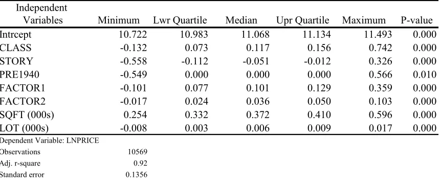
Table 6 contains the results of the GWR model. The adjusted R-squared4 improves to over 0.92 and the standard error declines to 0.136. This improvement reflects the
importance of localized spatial influences within the Tucson housing market. The GWR parameter estimates, which vary at each of the 10,569 observation points, are described by their median, minimum, and maximum value as well as interquartile range. In most cases, the parameter estimates from the global model are encapsulated within, or are very close to, the interquartile range of the GWR model. We note that pre 1940 vintage
4
housing is not present throughout much of the Tucson area, thus there is no variability at the majority of observation points which results in an interquartile range of zero.
Table 6. Model 4 Results: Geographically Weighted Regression Independent
Variables Minimum Lwr Quartile Median Upr Quartile Maximum P-value Intrcept 10.722 10.983 11.068 11.134 11.493 0.000 CLASS -0.132 0.073 0.117 0.156 0.742 0.000 STORY -0.558 -0.112 -0.051 -0.012 0.326 0.000 PRE1940 -0.549 0.000 0.000 0.000 0.566 0.010 FACTOR1 -0.101 0.077 0.101 0.129 0.359 0.000 FACTOR2 -0.017 0.024 0.036 0.050 0.103 0.000 SQFT (000s) 0.254 0.332 0.372 0.410 0.596 0.000 LOT (000s) -0.008 0.003 0.006 0.009 0.017 0.000
Dependent Variable: LNPRICE
Observations 10569 Adj. r-square 0.92 Standard error 0.1356
The parameter estimates for the seven independent variables vary widely over space. The P-value from a Monte Carlo significance test indicates that the spatial variation in all seven is significant at the .01 level or higher. This provides strong evidence that the marginal prices of these housing characteristics are not constant, but vary over space within the greater Tucson area.
The interquartile ranges of the GWR estimates are of plausible magnitudes, however, the minimum and maximum values are extreme or counter-intuitive in some cases. For example, the estimates for STORY range from -0.56 to 0.33, which implies that, all else equal, a multi-story house5 sells for 56% less than a single-story home at one regression point and 33% more at another. The PRE1940 estimates range from -0.549 to 0.566. Negative values for the CLASS and LOTSIZE coefficients, too, are counterintuitive, as they indicate that homes of low structural quality sell for more than those with higher structural quality at some locations and that an additional square foot of lot reduces price in some areas. The negative estimates, however, are statistically significant within only a very small portion of the study area.
5.2 Spatial patterns
One advantage of GWR is that the spatial patterns inherent in the parameter estimates can be easily mapped and visualized. The dwelling size (SQFT) estimates are shown in Figure 2. As expected, the estimates are positive and significant throughout the Tucson area and exhibit relatively smooth spatial trends. The highest marginal-price estimates are found within Central Tucson, where homes tend to be among the market’s smallest. The estimates also tend to be high in the exclusive Catalina Foothills area where demand
5
for large homes is great. The marginal price of an additional square foot of living space is generally low near the eastern and southern peripheries where homes are typically larger. In the northwest, the SQFT estimates exhibit a more localized pattern.
Figure 2. GWR SQFT parameter estimates
The spatial pattern of the LOTSIZE estimates is distinctly different from that of SQFT (Figure 3). The marginal-price estimates are generally positive, though not significant at the .05 level, throughout much of the central and southern portions of the Tucson area. The estimates tend to be highest in the northwest and southeast areas. Surprisingly, a large pocket of negative estimates is evident within a portion of the Catalina Foothills area, which indicates a possible misspecification problem. One might expect lower marginal prices in this area because lots are generally among the market’s largest, but it is difficult to explain why the marginal price of an additional square foot of lot would be negative. This is most likely attributable to characteristics that larger lot homes in this area have in common but are not included in the model.
Figure 3. GWR LOTSIZE parameter estimates
The estimates for several variables reflect complex, localized spatial patterns. For instance, while the coefficient for the STORY variable is negative and significant in the global model, the GWR parameter estimates indicate that ceteris paribus, multi-story homes sell for more than single story homes within a large area east of Central Tucson (Figure 5). High negative estimates for STORY are found just to the south of this area. Thus the GWR results suggest that the value of a multistory home is dependent upon locational context.
Figure 4. GWR STORY parameter estimates
5.3 Predictive accuracy
In order to assess the predictive accuracy of the GWR and the spatial expansion
approaches, predicted prices were estimated for the 10% of sales withheld from the initial models. In GWR, this is accomplished by estimating new models at the 1163 holdback sample locations using only the data from the original 10,569 observations. The
holdback sample analysis indicates that allowing housing attribute prices to vary with absolute location strengthens house price prediction accuracy.
10 percent 20 percent R-squared Model 1: Global 57.1 82.6 0.832 Model 2: Expansion 59.3 85.2 0.867 Model 3: Expansion with lag 59.3 86.7 0.882
[image:16.612.89.499.109.189.2]Model 4: GWR 64.6 88.3 0.878
Table 7. Out of sample predictive accuracy: Percent of predicted prices within specified range of actual price and R-squared between actual and predicted price
6 Discussion
Our results show that both the spatial expansion and GWR methods of incorporating spatial heterogeneity result in an improvement in explanatory power and predictive accuracy over the stationary coefficient model. The results also provide strong evidence for the presence of spatial heterogeneity within the Tucson market, indicating that the marginal prices of key housing attributes are not constant but vary with locational context.
GWR outperforms the spatial expansion method in terms of explanatory power and predictive accuracy. This difference is narrowed to some degree with the addition of the spatial lag term in the expansion specification. While the spatial expansion model is capable of picking up broad trends in the spatial structure of the housing parameters, GWR appears to be better able to represent the complex spatial patterns inherent in the Tucson data. This suggests that spatial heterogeneity may be due to discrete, localized influences, as well as those operating in a broad, continuous manner over space. Our results suggest that when explanatory power and predictive accuracy are the primary objectives, GWR is the superior approach.
A comparison of the absolute value of the GWR and spatial expansion residuals (Model 3) is depicted in Figure 5. Dark points represent locations where the GWR prediction was closer to the actual sale price, while light points indicate locations where the spatial expansion model was more accurate. Locations with similar absolute prediction errors (within .05) are suppressed. In general, GWR is more accurate within Central Tucson, where housing tends to be dense and heterogeneous, as well as near the periphery of the study area. The spatial expansion predictions tend to be more accurate within the area immediately surrounding the central core.
Figure 5. Comparison of absolute prediction error for the GWR and spatial expansion models
its ability to accommodate a larger number of variables and interactions. The expansion framework is also more conducive to hypothesis testing than is GWR.
Do the complex spatial trends depicted by GWR reflect true spatial variation in the price of the seven housing attribute variables? As argued earlier, there is good reason to expect variation in marginal prices within a large, dispersed market such as Tucson due to localized supply and demand dynamics, and the spatial pattern of the SQFT estimates appear to be plausible given our knowledge of the market. It is also plausible that the value associated with a multi-story house may vary with locational context. For example, in a neighborhood with desirable views and widely spaced homes, a multi-story home may be perceived as amenity. Conversely, a multi-story home may be perceived as a disamenity in an area with densely packed homes surrounded by less desirable land uses. If this is indeed the case, the stationary coefficient model has obscured this important relationship.
The negative estimates for LOTSIZE and CLASS are difficult to rationalize and are almost certainly due to some form of misspecification. Farber and Yeats (2006) found a similar result for several variables in their study of Toronto. Omitted variables in particular likely influence our results. While both the GWR and spatial expansion models incorporate absolute measures of location, neither includes direct measures of the neighborhood, environmental, and accessibility attributes that underpin the value of ‘location’. If these influences are not adequately controlled for through absolute location and are spatially correlated with variables included in the models, they may contribute to the observed spatial heterogeneity. This holds true for structural attributes as well. Consequently, GWR may provide a means to identify such misspecification problems.
A potential limitation of both the spatial expansion and GWR models is that they in essence impose a continuous pattern on the spatial structure of the market. However, it is widely recognized that some locational attributes that might lead to spatial heterogeneity are discrete in nature. For example, school districts are known to play an important role in the determination of housing prices. Therefore, one would expect price shifts to be abrupt when moving across the boundary from a high quality school district to a lower quality district. If this is the case, it may be more appropriate to delineate housing submarkets.
The expansion method can incorporate discrete effects by including submarket or neighborhood interaction terms (Fik, Ling, and Mulligan 2003). However, this may not be practical in some situations as it would result in an even greater number of
independent variables and require a priori knowledge of submarket boundaries. While it would be difficult to incorporate discrete influences in a GWR model, GWR may be a useful tool to determine whether segmentation is warranted as well as an aid in
7 Conclusions
Our comparison of the GWR and spatial expansion methods provides strong evidence that the marginal prices of key housing attributes are not constant throughout the Tucson market area, but vary with locational context. The parameter estimates for all seven housing attributes exhibited significant spatial variation in both models. We believe our results reflect both true variation in the marginal prices of these attributes due to localized supply and demand dynamics as well as potential misspecification problems such as omitted variables.
While both the spatial expansion and GWR approaches improve upon the results of the stationary coefficient model, GWR outperformed the spatial expansion specification in terms of explanatory power and predictive accuracy. The GWR results indicate that the spatial pattern of coefficient estimates is more complex than can be accounted for by a spatial expansion employing a third degree polynomial expansion of the homes’ {x, y} coordinates.
Regardless of whether the results are indicative of true parameter variation or
misspecification, they highlight the complex spatial structure of housing markets and the need to explicitly address spatial heterogeneity in housing market models. A failure to do so may result in a loss of explanatory power, lead to erroneous conclusions, and obscure important housing market dynamics. GWR in particular provides a means to visualize the spatial structure of housing markets. Either method may be a viable alternative in situations where price prediction is the primary concern and locational information is difficult to obtain or when knowledge of local submarkets is unavailable.
References
Agterberg F (1984) Trend surface analysis. In Spatial Statistics and Models, eds. Gale and Willmott, D. Reidel Publishing Co., pp. 147-171.
Anselin L (1988) Spatial econometrics, methods and models. Kluwer Academic, Dordrecht Boston London
Anselin L (1990) Spatial dependence and spatial structural instability in applied regression analysis. Journal of Regional Science 30: 185-207
Bourassa S, Hoesli M, Peng V (2003) Do housing submarkets really matter? Journal of Housing Economics 12: 12-28
Bowen W, Mikelbank B, Prestegaard D (2001) Theoretical and empirical considerations regarding space in hedonic housing price model applications. Growth and Change 32: 466-490
Brunsdon C, Fotheringham S, Charlton M (1996) Geographically weighted regression: A method for exploring spatial nonstationarity. Geographical Analysis 28: 281-298
Cassetti E (1972) Generating models by the expansion method: Applications to geographical research. Geographical Analysis 4: 81-92
Can A (1992) Specification and estimation of hedonic house price models. Regional Science and Urban Economics 22: 453-474
Can A, Mogbolugbe, I (1987) Spatial dependence and house price index construction.
Journal of Real Estate Finance and Economics 14: 203–222
Clapp, J (2001) A semi parametric method for valuing residential locations: applications to automated valuation. Journal of Real Estate Finance and Economics 27: 303-320
Dubin, R, Sung C (1987) Spatial variation in the price of housing: Rent gradients in non-monocentric cities. Urban Studies 24: 193-204
Farber S, Yates M (2006) A Comparison of Localized Regression Models in an Hedonic Price Context, Canadian Journal of Regional Science (forthcoming)
Fik T, Ling D, Mulligan G (2003) Modeling spatial variation in housing prices: A variable interaction approach. Real Estate Economics 31: 623-646
Fotheringham A, Brunsdon C, Charlton N (2000) Quantitative geography: Perspectives on spatial data analysis. Sage Publications, London
Fotheringham A, Brunsdon C, Charlton N (2002) Geographically weighted regression: The analysis of spatially varying relationships. John Wiley, Chichester
Freeman A (2003) The measurement of environmental and resource values. Resources for the Future, Washington D.C.
Goodman A (1981) Housing submarkets within urban areas – definitions and evidence.
Journal of Regional Science 21: 175-185
Goodman A (1998) Housing market segmentation. Journal of Housing Economics 7: 121-143
Jones J, Cassetti, E (1992) Applications of the expansion method. Routledge, London
Michaels R, Smith V (1990) Market segmentation and valuing amenities with hedonic models: The case of hazardous waste sites. Journal of Urban Economics 28: 223-242.
Mulligan G, Franklin R, Esparaza A (2002) Housing prices in Tucson, Arizona. Urban Geography 23: 446-470
National Association of Realtors (2006) Single-family spreadsheet. Chicago, IL
Ordford S (1999) Valuing the built environment: GIS and house price analysis. Ashgate, Aldershot
Pavlov A (2000) Space-varying regression coefficients: A semi-parametric approach applied to real estate markets. Real Estate Economics 28: 249-283
Páez, A (2005) Local Analysis of Spatial Relationships: A Comparison of GWR and the Expansion Method, Lecture Notes in Computer Science, 3482, 162-172
Páez, A, Uchida, T, Miyamoto, K (2001) Spatial Association and Heterogeneity Issues in Land Price Models, Urban Studies, 38 (9) 1493-1508.
Schnare A, Struyk R (1976) Segmentation in urban housing markets. Journal of Urban Economics 4: 146-166.
Quigley J (1985) Consumer choice of dwelling, neighborhood and public services.
Regional Science and Urban Economics 15: 41-63
Appendix 1
[image:21.612.90.525.210.358.2]A principal component analysis was performed in order to reduce the number of explanatory variables while mitigating potential omitted variables bias. Eight housing attributes were entered into the PCA. Our objective was to reduce these variables to as few factors as possible due to computational limitations imposed by GWR. We retained the two components with eigenvalues greater than one for use in the regression models (Table 10), which together explain 56% of the variance in the original eight variables.
Table 9. Total Variance Explained
Percent of Cumulative Percent of Cumulative Component Total variance percent Total variance percent
1 2.972 37.152 37.152 2.860 35.751 35.751 2 1.510 18.879 56.031 1.622 20.280 56.031 3 0.916 11.453 67.484
4 0.813 10.158 77.642 5 0.704 8.805 86.448 6 0.457 5.707 92.154 7 0.362 4.529 96.683 8 0.265 3.317 100.000
Extraction Method: Principal Component Analysis.
Initial Eigenvalues Rotation Sums of Squared Loadings
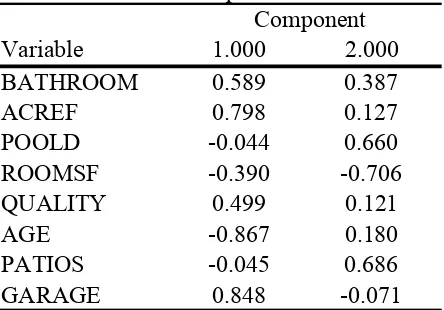
The extracted components were rotated via the varimax method with kaiser normalization (Table 11). Component one loads negatively on age, and positively on refrigerated air conditioning, enclosed garages and number of bathroom fixtures per room in the home. This component represents homes with modern features. We expect a positive
relationship between this factor and housing prices. Component two has a high negative loading on the number of rooms per square foot of living space (large rooms), and positive loadings on homes with pools and patios. This component represents a specific style of housing, with a spacious design and outdoor amenities. A positive association between this component and housing prices is anticipated.
Table 10. Rotated Components
Variable 1.000 2.000 BATHROOM 0.589 0.387 ACREF 0.798 0.127 POOLD -0.044 0.660 ROOMSF -0.390 -0.706 QUALITY 0.499 0.121
AGE -0.867 0.180
PATIOS -0.045 0.686 GARAGE 0.848 -0.071
Rotation Method: Varimax with Kaiser Normalization.
[image:21.612.92.314.536.691.2]