http://dx.doi.org/10.4236/ijg.2014.58068
A Method to Estimate Spatial Resolution in
2-D Seismic Surface Wave Tomographic
Problems
Jorge L. de Souza
Coordenação de Geofísica, MCTI/Observatório Nacional, Rio de Janeiro, Brazil Email: [email protected]
Received 15 May 2014; revised 12 June 2014; accepted 5 July 2014
Copyright © 2014 by author and Scientific Research Publishing Inc.
This work is licensed under the Creative Commons Attribution International License (CC BY).
http://creativecommons.org/licenses/by/4.0/
Abstract
A novel methodology to quantify the spatial resolution in 2-D seismic surface wave tomographic problems is proposed in this study. It is based on both the resolving kernels computed via full res-olution matrix and the concept of Full Width at Half Maximum (FWHM) of a Gaussian function. This method allows estimating quantitatively the spatial resolution at any cell of a gridded area. It was applied in the northeastern Brazil and the estimated spatial resolution range is in agreement with all previous surface wave investigations in the South America continent.
Keywords
Surface Waves, Seismic Tomography, Wave Propagation, Spatial Resolution, Northeastern Brazil
1. Introduction
A regionalized dispersion curve at each cell of the grid was then used to estimate the 1-D S-velocity in depth. The spatial resolution was obtained through both checkerboard and realistic structure tests. According to [2], the spatial resolution at 30 km is around 4˚, while at 100 km it is 6˚ and at 150 km it is 8˚. The general features of the S wave velocities anomalies at those depths were presented and discussed. More recently, [3] used joint in-version of waveforms and fundamental mode Rayleigh wave group-velocities to investigate the South America continent. The methodologies used by both [1][2] were used in this study to get group-velocities and for wave-forms inversions, respectively. The spatial resolution was obtained with checkerboard tests and according to the authors it was 6˚ at both 100 and 300 km depths. The S wave velocities anomalies to these depths were pre-sented and discussed. The most recent study about the S wave velocity structure beneath South America conti-nent was presented by [4]. He used a group of 128 earthquakes occurred at western South America continent and recorded by 71 seismic stations distributed throughout continental part of the region. Rayleigh wave group-ve- locities varying from 5 to 250 s were used to obtain the source-station dispersion curves. The region was divided into cells of 4˚ × 4˚ and a regionalized Rayleigh wave dispersion curve was obtained for each cell of the grid. Each regionalized dispersion curve was inverted to get a 1-D S wave velocity in each cell. None quantitative evaluation about spatial resolution of the estimated shear wave velocity in the region was presented. Only a qua-litative evaluation of the resolution (i.e., the terms bad resolution and poor resolution were applied to classify the resolution in depth) was presented and discussed. In the present study, a mathematical approach to estimate quantitatively the spatial resolution in 2-D seismic surface wave problems is proposed and it is applied in the northeastern Brazilian region.
2. The Two-Dimensional Surface Wave Tomographic Problem
Let’s consider an area, defined by a pair of geographycal coordinates, which is discretized into square cells. Suppose that there are m source-station surface wave paths crossing this area and also assume that for a par-ticular path, the total source-station surface wave travel time is the sum of the travel time in each cell. Thus, for an th
i path and a given period
( )
T , one can write [5]( )
( )
1( )
( )
1 1 n 1 1
ij j
i i i j j
d
U T V T = D u T v T
− = −
∑
(1)where v Tj
( )
is an attributed phase and/or group velocity for the jth cell, V Ti( )
is the source-station phase and/or group velocity for the ith path calculated from attributed v Tj( )
, U Ti( )
is the observed source-sta- tion phase and/or group velocity for the ith path, u Tj( )
is the phase and/or group velocity for the jth cell,ij
d is the length of the ith path in the jth cell, and Di is the source-station distance of the ith path. The result of the procedure aforementioned is a dispersion curve (phase and/or group velocity as a function of period) for each cell of the target area. It is also important to remember that only the cells visited by at least one surface wave path are considered in such computation. Equation (1) can be rewritten in a matrix form as
=
y Ax (2)
where y is a residual vector (m × 1), x is a vector with the unknown parameters (n × 1) and A is a mxn matrix relating model parameters to observations. In terms of damped least-squares [6] [7], Equation (2) is given by
(
T 2)
−1 T= +
x A A θ I A y (3)
where AT is the transpose of matrix A, θ2 is the Levenberg-Marquardt parameter, and I is the identity matrix. In this context, the expressions for resolution
( )
R and covariance( )
C matrices are the following(
T 2)
−1 T= +
R A A θ I A A (4)
(
)
1(
)
12 T 2 T T 2
σ
− −= + +
C A A θ I A A A A θ I (5)
resolving kernels. The standard deviations of the estimated group-velocities at each cell are obtained in the di-agonal elements of the covariance matrix. Furthermore, several factors can contribute to uncertainties in group-velocity estimation [8]. These include origin time error, epicenter mislocation error, source finiteness er-ror, rise time erer-ror, etc. These errors were estimated and incorporated to the
σ
2 term of the covariance matrix( )
C .3. Estimation of the Spatial Resolution
The best and more accurate way of getting the resolution of the estimated phase and/or group velocities in any place of the earth’s planet, i.e., the spatial extent of the smallest phase and/or group velocity anomaly that can be imaged, is through the computation of resolution matrix. However, the computation of this matrix is not a simp-ly task, because it involves operations with very large matrices. For this reason, the major part of these kinds of studies does not compute the resolution matrix. In general, those studies use a different approach, called check-erboard tests, which are based on the inversion of synthetic data constructed as from subjective assumptions about input and output models [9] According to [9], in such analysis the quality criterion is the similarity be-tween both final and initial models used to calculate the synthetics.
In this study, we calculated the exact resolution matrix (Equation (4)), by using some efficient computational techniques into a Personal Computer [10]. It is fundamental to observe that the computation of the resolution matrix through Equation (4) is based only on the surface wave paths distributions of the target area.
According to [11], if the resolution has a single sharp maximum centered about the main diagonal, thus the data are well resolved. However, if the resolution is very broad, thus the data are poorly resolved (Section 4.2 of [11]). In spite of these important definitions, none way of quantifying the resolution is presented in the seismo-logical literature.
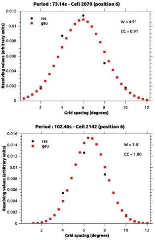
In this study, a novel methodology to quantify the spatial resolution in 2-D seismic surface wave tomographic problems is proposed. It is based on both the resolving kernels obtained via computation of the full resolution matrix (Equation (4)) and a basic property of a Gaussian function, because a resolving kernel shape can be ap-proximated to a Gaussian function. In fact, as θ2 in Equation (4) is always a positive number, then the lines of
R assume a maximum value in the position of the unknown parameter under evaluation (i.e. phase and/or group velocity at a particular cell) and the neighborhoods points tend to zero. A graphical representation of such resolving kernel shows that it follows a Gaussian function. Thus, by using this assumption and the concept of Full Width at Half Maximum (FWHM) of a Gaussian function, which represents the difference between the two values of the independent variable at which the dependent variable is equal to half of its maximum value [12]. In spectroscopy, the concept of FWHM of a Gaussian function is applied in the definition of spectrometers’ resolu-tion [13]-[14].
According to [15], the FWHM of a Gaussian function is given by
FWHM=2.35482σ (6)
where σ is the standard deviation. Thus, let’s consider a Gaussian function described by the following expres-sion
( )
221 exp
2 2π
x f x
σ σ
= −
(7)
where x is the independent variable and σ was defined previously. Then, rewriting Equation (7) in a con-densed way
2 exp
y=b cx (8)
where y is equal to f x
( )
and1 2π b
σ
= (9)
2
1
2 c
σ
= − (10)
Applying the natural logarithm in both sides of Equation (8)
2
lny=lnb cx+ (11)
The Equation (11) is a second order polynomial function or a quadratic function, which is represented graph-ically by a parabola. In this case, a quadratic least-squares fit can be used to get the three coefficients of the qu-adratic function and, consequently, the parameter c.
Extracting σ from Equation (10), we get
1
2 c
σ
=⋅ − (12)
Substituting Equation (12) in Equation (6), one gets an expression for the width of the Gaussian at half max-imum
( )
W as a function only of the parameter c, which is given by2.35482 2 W
c =
⋅ (13)
Equation (13) provides a quantitative spatial resolution measurement of the unknown parameter at any cell of the grid under investigation. Here, the unknown parameter is the estimated phase and/or group velocity either at a specific cell or at a particular period (Equation (1)). As the periods of the surface waves dispersion curves are related to depths (i.e. short periods are associated with shallow depths while long periods are related to deep parts of the earth’s interior), then the Equation (13) also allows the evaluation of the spatial resolution in depth.
The Equation (4) shows that the resolution matrix is a square matrix, i.e., if the number of unknown parame-ters is p, then R has p×p elements. As each element of a resolving kernel is related to the phase and/or group velocity at a given cell, then each element of R matrix has a spatial location, because it is represented by the geographical coordinates. Furthermore, if a resolving kernel has a shape similar to a Gaussian function [11], thus the maximum value of it should be located at the cell (i.e. the center of it) under investigation and it should decay to zero around a central value. I am interested in analyzing the spatial shape of the resolving ker-nel around a specific cell, i.e., the spread of the resolution or spatial decay around a central point, which is lo-cated in the diagonal of the resolution matrix [11].
4. Application to the Northeastern Brazilian Region
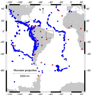
The region limited by the geographical coordinates (−125, 45) and (25, −75) is, initially, divided into square cells of 2˚ × 2˚ (Figure 1). To have a good path coverage of the target area (i.e., northeastern Brazil), a large quantity of earthquakes recorded at twenty three seismic stations (from 1988 to 1998 [16]) of the IRIS Consor-tium [17], located either in or around South America continent, were selected in this study.
The digital seismograms, related to seismic events with focal depth shallower than 120 km and magnitude higher than 5.0 mb, were requested and received from IRIS. The Seismic Analysis Code (SAC) package [18] was used to the identification of the surface waves in the seismic signals. This analysis produced 3134 digital seismograms, corresponding to 1082 earthquakes (Figure 1). The vertical components of the motion were used here and they represent 3134 source-station Rayleigh wave paths in the area displayed in Figure 1. To remove the effect of the seismograph on the seismic signal, an instrumental correction was applied in the seismograms (via SAC). Correction for source group delay was not applied, because it is considered a small source of error [19]. The Multiple-Filter Technique [20] was applied in the digital seismograms selected for this study. Twenty two periods, ranging from 10 to 102 s (i.e., 10.04, 12.05, 14.03, 16.00, 18.29, 20.08, 24.38, 28.44, 32.00, 36.57, 42.67, 46.55, 51.20, 56.89, 60.24, 64.00, 68.27, 73.14 78.77, 85.33, 93.09, 102.40 s), were selected to compose the source-station dispersion curves. This computation produced 3134 source-station Rayleigh wave group ve-locity dispersion curves and all details about the surface wave data processing can be found in [16].
Figure 1.Seismic stations (red triangles) and epicenters of the earthquakes (blue cir-cles) used in the present study. The area is limited by the geographical coordinates (−125, 45) and (25, −75). The heavy square box represents northeastern Brazilian re-gion.
investigate northeastern Brazilian region, thus we selected only the Rayleigh wave dispersion curves associated with each cell of such region (Figure 2). For each period, its source-station Rayleigh wave path distributions were plotted into maps to give an idea about their spatial distribution (Figures 3-7).
5. Discussion of the Results
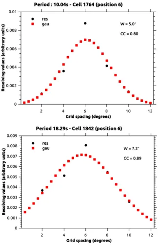
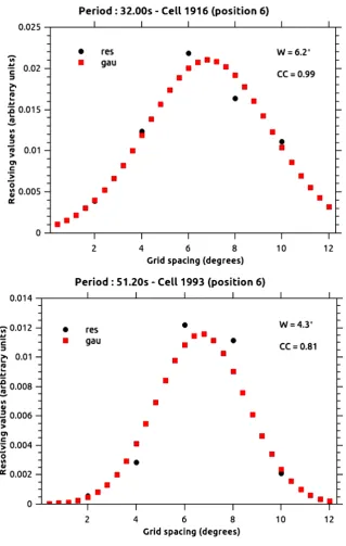
The width of the Gaussian at half maximum (W—Equation (13)) was used to get the spatial resolution of the es-timated Rayleigh wave group-velocities at each cell of the northeastern Brazil. As the region under investigation is formed by 49 cells (Figure 2) and each cell has a dispersion curve (which is composed of 22 periods), I got 1078 resolution estimates (49 × 22) for the northeastern Brazilian region. All those results are condensed in
Table 1. For a given cell of the northeastern Brazilian region, I got five elements of the resolution matrix (Equa-tion (4)). The central point (third element) is related to the center of the cell under evalua(Equa-tion and the others four points are located in the centers of the neighborhood cells (two on left and two on right). Here, the separation between each central point is equal to 2˚, because the studied area was divided into cells of 2˚ × 2˚, thus the se-paration between the five points is equal to 2˚.
Figure 2. The grid of the Figure 1 was divided into cells of 2˚ × 2˚ and each cell on it was numbered (from top to bottom and from left to right) so that any region inside northeastern Brazil must be associated with the numbers shown on the map.
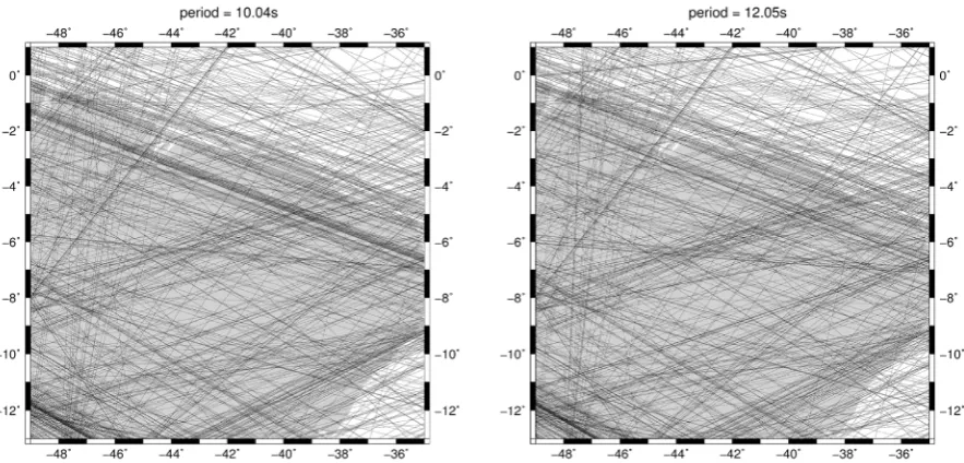
Figure 3.Source-station Rayleigh wave path distributions (for periods of 10.04 and 12.05 s) in the area of the northeastern Brazil. The black lines are the great-circle paths connecting epicenters and stations. The target area is relatively well covered by the Rayleigh wave path distribution. A clear decrease in the quantity of the source-station paths, when the period increas-es, is observed in these maps.
[image:6.595.93.535.404.616.2]Figure 4. Source-station Rayleigh wave path distributions (for periods of 16.00 and 20.08 s) in the area of the northeastern Brazil. The black lines are the great-circle paths connecting epicenters and stations. The target area is relatively well covered by the Rayleigh wave path distribution. A clear decrease in the quantity of the source-station paths, when the period increas-es, is observed in these maps.
Figure 5.Source-station Rayleigh wave path distributions (for periods of 24.38 and 32.00 s) in the area of the northeastern Brazil. The black lines are the great-circle paths connecting epicenters and stations. The target area is relatively well covered by the Rayleigh wave path distribution. A clear decrease in the quantity of the source-station paths, when the period increas-es, is observed in these maps.
shows that 70% of them are equal and higher than 0.7. The large quantity of high CC values indicates that Gaus-sian function seems to be a good representation of the resolving kernels’ shape.
[image:7.595.95.535.358.589.2]Figure 6.Source-station Rayleigh wave path distributions (for periods of 46.55 and 68.27 s) in the area of the northeastern Brazil. The black lines are the great-circle paths connecting epicenters and stations. The target area is relatively well covered by the Rayleigh wave path distribution. A clear decrease in the quantity of the source-station paths, when the period increas-es, is observed in these maps.
Figure 7. Source-station Rayleigh wave path distributions (for periods of 85.33 and 102.40 s) in the area of the northeastern Brazil. The black lines are the great-circle paths connecting epicenters and stations. The target area is relatively well covered by the Rayleigh wave path distribution. A clear decrease in the quantity of the source-station paths, when the period increas-es, is observed in these maps.
Table 1 also shows that the group-velocity anomalies smaller than 3.2˚ cannot be resolved in northeastern Brazil and, therefore, those anomalies should not be considered in the spatial resolution analysis. It is important to emphasize that the procedure developed here allows analyzing any group velocity anomaly in any particular point of the area studied.
decrease in a spatial resolution) or an almost constant throughout the entire period range (or depth range) dis-played in Table 1. In some cases (cells 1840, 2141 and 2142, Table 1), the spatial resolution values increase when the period increases. In these cases, we can observe two main regions on Table 1 (i.e., periods lower than 46.55 s and periods higher than 46.55 s). In the first region (periods ≤ 46.55 s), the spatial resolution values are higher than those for the second region (periods > 46.55 s). As shown inTable 1 and expected, it seems that azimuthal distribution is a parameter more important than the quantity of the surface wave paths. These results indicate that it is possible to get a better spatial resolution by using a reduced quantity of seismic data.
Another important point observed in the proposed methodology is related to the improvement of the spatial resolution in surface wave tomography studies. In general, in the major part of the surface wave studies in the seismological literature, the improvement of spatial resolution is associated with the increase of data quantity. In fact, the improvement of the spatial resolution should be related to the cell size. Let’s consider the case of a photo. In order to increase the resolution of a photo we must decrease the size of the discretization element, i.e., in this case, we increase the number of dots per inch (or increase the density of dots and, consequently, decrease the dot size). Thus, to get a better spatial resolution we must either decrease the cell size or increase the number of source-station paths with a good azimuthal coverage. The previous discussions show that the proposed me-thodology describes the main features of the seismological problem.
6. Conclusion
A novel methodology to quantify the spatial resolution in 2-D seismic surface wave tomographic problems is proposed. It is based on both the resolving kernels computed via full resolution matrix and the concept of Full Width at Half Maximum (FWHM) of a Gaussian function. The method allows estimating quantitatively the spa-tial resolution at any cell of a gridded area. The spaspa-tial resolution range estimates with the proposed method in northeastern Brazil is in agreement with those obtained with all previous surface wave investigations in the South America continent.
Acknowledgements
This research was developed by using data from GSN and GTSN seismic networks available at IRIS. The author would like to thank these institutions for providing all seismic data. He also thanks Fundação de Amparo à Pes-quisa do Estado do Rio de Janeiro (FAPERJ) for financial support during the development of this study (Process #: E-26/170.407/2000) and MCTI/Observatório Nacional for all support. Several figures were prepared with the software Generic Mapping Tools [24].
References
[1] van der Lee, S., James, D. and Silver, P. (2001) Upper Mantle S Velocity Structure of Central and Western South Am- erica. Journal of Geophysical Research, 106, 30821-30834. http://dx.doi.org/10.1029/2001JB000338
[2] Feng, M., Assumpção, M. and van der Lee, S. (2004) Group-Velocity Tomography and Lithospheric S-Velocity Structure of the South American Continent. Physics of the Earth and Planetary Interiors, 147, 315-331.
http://dx.doi.org/10.1016/j.pepi.2004.07.008
[3] Feng, M., van der Lee, S. and Assumpção, M. (2007) Upper Mantle Structure of South America from Joint Inversion of Waveforms and Fundamental Mode Group Velocities of Rayleigh Waves. Journal of Geophysical Research, 112, B04312. http://dx.doi.org/10.1029/2006JB004449
[4] Corchete, V. (2011) Shear-Wave Velocity Structure of South America from Rayleigh-Wave Analysis. Terra Nova, 24, 87-104. http://dx.doi.org/10.1111/j.1365-3121.2011.01042.x.
[5] Feng, C.-C. and Teng, T.-L. (1983) Three-Dimensional Crust and Upper Mantle Structure of the Eurasian Continent.
Journal of Geophysical Research, 88, 2261-2272. http://dx.doi.org/10.1029/JB088iB03p02261
[6] Aki, K. and Richards, P.G. (1980) Quantitative Seismology. 1st Edition, Freeman, San Francisco, 932.
[7] Lines, L.R. and Treitel, S. (1984) Tutorial: A Review of Least-Squares Inversion and Its Application to Geophysical Problems. Geophysical Prospecting, 32, 159-186. http://dx.doi.org/10.1111/j.1365-2478.1984.tb00726.x
[8] Cloetingh, S., Nolet, G. and Wortel, R. (1979) On the Use of Rayleigh Wave Group Velocities for the Analysis of Continental Margins. Tectonophysics, 59, 335-346. http://dx.doi.org/10.1016/0040-1951(79)90054-4
http://dx.doi.org/10.1111/j.1365-246X.1993.tb05605.x
[10] Dos Santos, N.P. and de Souza, J.L. (2005) Aplicação de eficientes técnicas computacionais a problemas de tomografia sísmica com ondas superficiais. Revista Brasileira de Geofísica, 23, 285-294.
[11] Menke, W. (1989) Geophysical Data Analysis: Discrete Inverse Theory. 1st Edition, Academic Press, San Diego, 289.
[12] Wikipedia. Full Width at Half Maximum. http://en.wikipedia.org/wiki/Full_width_at_half_maximum.
[13] Herbert, C.G. and Johnstone, R.A.W. (2002) Mass Spectrometry Basics. 1st Edition, CRC Press, Boca Raton, 453.
[14] De Hoffmann, E. and Stroobant, V. (2007) Mass Spectrometry: Principles and Applications. 1st Edition, John Wiley & Sons, England, 489.
[15] Weisstein, E. (2014) Wolfram Math World, Gaussian Function. http://mathworld.wolfram.com/GaussianFunction.html
[16] Vilar, C.S. (2004) Estrutura tridimensional da onda S na litosfera do nordeste brasileiro. Ph.D. Thesis, MCTI/ Observatório Nacional, Rio de Janeiro, Brazil.
[17] Butler, R., Lay, T., Creager, K., Earl, P., Fischer, K., Gaherty, J., Laske, G., Leith, B., Park, J., Ritzwoller, M., Tromp, J. and Wen, L. (2004) The Global Seismographic Network Surpasses Its Design Goal. Eos, Transactions American Geophysical Union, 85, 225-229. http://dx.doi.org/10.1029/2004EO230001
[18] Goldstein, P., Dodge, D., Firpo, M. and Minner, L. (2003) SAC2000: Signal Processing and Analysis Tools for Seis-mologists and Engineers. In: Lee, W.H.K., Kanamori, H., Jennings, P.C. and Kisslinger, C., Eds., The IASPEI Interna-tional Handbook of Earthquake and Engineering Seismology, Academic Press, London, 1613-1614.
http://dx.doi.org/10.1016/S0074-6142(03)80284-X
[19] Levshin, A.L., Ritzwoller, M.H. and Resovsky, J.S. (1999) Source Effects on Surface Wave Group Travel Times and Group Velocity Maps. Physics of the Earth and Planetary Interiors, 115, 293-312.
http://dx.doi.org/10.1016/S0031-9201(99)00113-2
[20] Dziewonski, A., Bloch, S. and Landisman, M. (1969) A Technique for the Analysis of Transient Seismic Signals. Bul-letin of the Seismological Society of America, 59, 427-444.
[21] Silveira, G., Stutzmann, E., Griot, D.-A., Montagner, J.-P. and Victor, L.M. (1998) Anisotropy Tomography of the At-lantic Ocean from Rayleigh Surface Waves. Physics of the Earth and Planetary Interiors, 106, 257-273.
http://dx.doi.org/10.1016/S0031-9201(98)00079-X
[22] Vdovin, O., Rial, J.A., Levshin, A.L. and Ritzwoller, M.H. (1999) Group-Velocity Tomography of South America and the Surrounding Oceans. Geophysical Journal International, 136, 324-340.
http://dx.doi.org/10.1046/j.1365-246X.1999.00727.x
[23] Silveira, G. and Stutzmann, E. (2002) Anisotropic Tomography of the Atlantic Ocean. Physics of the Earth and Plane-tary Interiors, 132, 237-248. http://dx.doi.org/10.1016/S0031-9201(02)00076-6
currently publishing more than 200 open access, online, peer-reviewed journals covering a wide range of academic disciplines. SCIRP serves the worldwide academic communities and contributes to the progress and application of science with its publication.
Other selected journals from SCIRP are listed as below. Submit your manuscript to us via either