Effects of Easy Hybrid Parallelization with CUDA for OpenMX

Effects of Easy Hybrid Parallelization with CUDA for

OpenMX

Jae-Hyeon Parq

QoLT IIDC and School of Earth and Environmental Sciences,

Seoul National University, Seoul 151-747, Korea

Erik Sevre

QoLT IIDC and School of Earth and Environmental Sciences,

Seoul National University, Seoul 151-747, Korea

Sang-Mook Lee

QoLT IIDC and School of Earth and Environmental Sciences,

Seoul National University, Seoul 151-747, Korea

ABSTRACT

A MPI-friendly density functional theory (DFT) source code was modified within hybrid parallelization including CUDA. The objective is to find out how simple conversions within the hybrid parallelization with mid-range GPUs affect DFT code not originally suitable to CUDA. Several rules of hybrid parallelization for numerical-atomic-orbital (NAO) DFT codes were settled. The test was performed on a magnetite material system with OpenMX code by utilizing a hardware system containing 2 Xeon E5606 CPUs and 2 Quadro 4000 GPUs. 3-way hybrid routines obtained a speedup of 7.55 while 2-way hybrid speedup by 10.94. GPUs with CUDA complement the efficiency of OpenMP and compensate CPUs’ excessive competition within MPI.

General Terms

Parallel computing, Heterogeneous computing, Computational Chemistry.

Keywords

MPI, CUDA, OpenMP, electronic structure, graphical processing unit, pseudo-atomic-orbital

1.

INTRODUCTION

The density functional theory (DFT) is a quantum calculation tool widely used in material sciences. Compared to other quantum chemical methods, DFT prides itself on its low computational cost and moderate accuracy [1], which make DFT useful in recent theoretical research of large model systems consisting of many atoms. There are various DFT code packages classified by wavefunction basis sets; OpenMX [2] and SIESTA [3] are famous as code packages using numerical-atomic-orbital (NAO) basis sets. The keys to how DFT codes have succeeded in the last decades are adequate approximations and suitable parallelization with message-passing interface (MPI) [4].

Parallelization methods for newly developed computer architectures are becoming more important since research simulations need increasingly large model sizes. As high-end computer architectures have adopted cluster structures with memory distributed in nodes, MPI has been dominantly used due to its convenience to users. Development of multi-core architectures, however, has increased utilization of OpenMP [5], parallelism within shared memory systems. Recent high performance computing architectures have applied heterogeneous memory systems and inspired hybrid parallelism using both MPI and OpenMP [6].

Graphical processor units (GPUs) are improving so as to overcome the speed limit of CPUs in the name of general

purpose computing on GPUs (GPGPU) although cache-based CPUs are still very successful for speeding up the high-end supercomputers. The spirit of GPGPU is that GPUs assist CPUs and reduce total calculation time by converting some parts of an original CPU code into those optimal on GPUs. The early stage of GPGPU suffered from poor programmability and lack of double-precision compute capability. Programming for GPUs became easy with the introduction of NVIDIA’s Compute Unified Device Architecture (CUDA) [7], and the hardware problem disappeared with the release of NVIDIA’s state-of-the-art GPUs with double-precision instruction sets.

CUDA implementation has successfully accelerated DFT codes on plane-wave basis set [8] and on Gaussian basis set [9]. In the former [8], it is sufficient to utilize libraries distributed by NVIDIA and to rectify some code because the original CPU version code has full of easily converted parts. If it is not the case, the code should be greatly transformed to be fit for GPU. In the latter [9], the original code’s algorithm was changed to increase the efficiency on GPUs.

Each parallelism has its own advantages and disadvantages. MPI processes cannot share memory to require data transfer among processes. OpenMP and CUDA apply shared memories but must follow established forms in memory access to reduce conflicts among threads, which would occur less within MPI. CUDA’s available threads outnumber OpenMP’s, but a GPU device needs to transfer data with its host (CPUs). Neither CUDA nor OpenMP can combine computer nodes, but MPI can. Hybridization between these parallelisms means various kinds of parallelization need to undertake the difficult task to be combined in parts into a determined form, and there have been several successes of the hybrid parallelization with CUDA [10-17].

big problem, requiring changes in most of the code. Instead of all this work, hybrid parallelization with CUDA can be a compromise. The problem is whether the speedup from the hybrid parallel computation is comparable to that from changing the main algorithm. A test for the hybrid parallelization without changing the main algorithm is therefore needed.

This paper discusses strategies for hybrid parallelization on NAO DFT, and tests them to analyze their benefit. Parallelizable parts in DFT codes have certain specific patterns, varied by the basis set chosen. The next section investigates how to combine MPI, OpenMP and CUDA for NAO DFT calculation, by examining patterns from relevant DFT routines utilized. In the following section, the hybrid strategies are applied to OpenMX package [18] and it is judged whether the resulting speedup is meaningful.

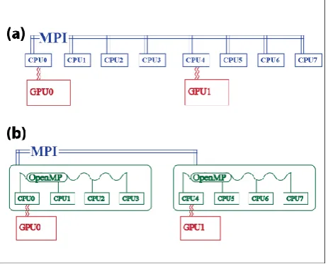
Fig 1: (Color online) Schematic pictures of hybrid parallelization candidates of (a) MPI+OpenMP+CUDA and (b) MPI+CUDA.

2.

HYBRID PARALLELIZATION

STRATEGIES FOR NAO DFT

Let’s first consider schematic hybrid parallelization in terms of hardware. To utilize all CPUs and GPUs, we naturally consider combining all three methods, OpenMP, MPI, and CUDA parallelization. When the number of GPU devices is less than that of CPU cores, one can easily devise a scheme to divide the GPU devices amongst the CPU cores. Each (OpenMP) master thread communicates with its assigned GPU device via CUDA and with other master threads via MPI, as described in Fig. 1 (a). This is similar to those suggested by some papers [12-15], but there are small differences in them such that GPU execution does not overlap CPU operation or all CPU cores do not participate in OpenMP organized work. In our scheme, if the number of CPU cores is four times to that of GPU devices, for example, OpenMP should bind every 4 CPU cores, connected to every single GPU within CUDA, and MPI connects each bunch of 4 CPU cores with the other CPU core bunches. This 3-way hybrid parallelization consumes less memory than parallelization without OpenMP since memory cost depends on the number of MPI processes, but it is not guaranteed that the resulting speed will surpass MPI only parallelization. Another way of organizing the hybrid parallelization is excluding the use of OpenMP to avoid some potential slowdowns and can be found in some literature [10]. This type of hybrid parallelization will be demanded if the speed of the above

3-way hybrid parallelization fails to exceed MPI only parallelization or if the contribution of OpenMP in the 3-way hybrid parallelization is too small. All CPU cores communicate with each other via MPI as shown in Fig. 1 (b). Only specific CPU cores are connected to GPU devices, i.e., nonequivalent allocation. Thus this parallelization scheme guarantees the speed higher than MPI only parallelization. In this case, however, load balancing among MPI processes is not trivial. The best way of distributing load to CPU cores is probably dynamic load balancing or determination by tests. With these two ideas on parallelization it is next necessary to analyze the DFT codes from the viewpoint of our hybrid parallelization schemes. Most of the focus will be on 3-way hybrid methods, since they appear to have the greatest potential for optimizations. In the case of the MPI+CUDA 2-way hybrid method, the assignment of tasks is based on changing the 3-way hybrid method by reassigning the parts based on OpenMP in the 3-way method to serial CPU parallelized using MPI or CUDA routines. The problem of choosing whether to implement serial or CUDA is not trivial, but it seems related to the problem of choosing whether to implement OpenMP or CUDA.

Large-scale parallelization usually concerns loops in a serial code, i.e., data parallelization, but task parallelization, requiring fixed number of processes or threads, is usually inappropriate for general cases of DFT codes, although OpenMP can handle it. Thus the priority is checking what loops are contained in a DFT code. Simply speaking, DFT calculation has a procedure of five parts [19], initial setting, calculating effective potential, diagonalization (solving eigenvalue equation), calculating densities and obtaining results. The middle three parts consist of the main iterated loop and spend the most of total calculation time. So we will focus on these three parts. The part to determine effective potential contains loops to calculate elements of the Hamiltonian matrix and the overlap matrix, both of which consist of the eigenvalue equation concerned by the diagonalization part. The charge density or spin density is calculated within loops for density grid.

Table 1. Key parameters of parallelizable loops in DFT calculation and their scales, considering usual large-scale

calculation.

Parameter Loop scale

k-points a _{O(1) ~ O(100)}

Atoms O(100) ~ O(1000)

Basis functions O(1000) ~ O(10000) Auxiliary basis functions a O(100000) ~ O(1000000)

a

If their arrays are one-dimensionalized.

Keeping in mind the loop indices, the parallelizable loops in a NAO DFT code were classified. The computation of effective potential and diagonalization concern the Hamiltonian matrix and the overlap matrix, but the former parts do not use the k-point index. These matrices are reducible and divided into respective k-point matrices (or spins). So diagonalization can be easily parallelized within MPI because matrices of disparate k-points (or spins) require little information communicated between nodes, i.e., close to embarrassing parallelism, which is one of reasons to make DFT codes MPI-friendly. On the other hand, k-point index can be ignored in the effective potential calculation part because adding k-point dependence is just multiplying a simple matrix and consumes little time. So MPI is not necessary for that calculation with respect to k-point index. For basis function index, shared memory parallelization should be better equipped to deal with the Hamiltonian matrix and the overlap matrix than MPI because those matrices are irreducible after they are separated into single k-point ones (within non-spin or non-collinear spin calculation [21], or with single spin within collinear spin calculation). For auxiliary basis functions, consisting of density grids used in calculating effective potential or densities, shared memory parallelization looks more appropriate.

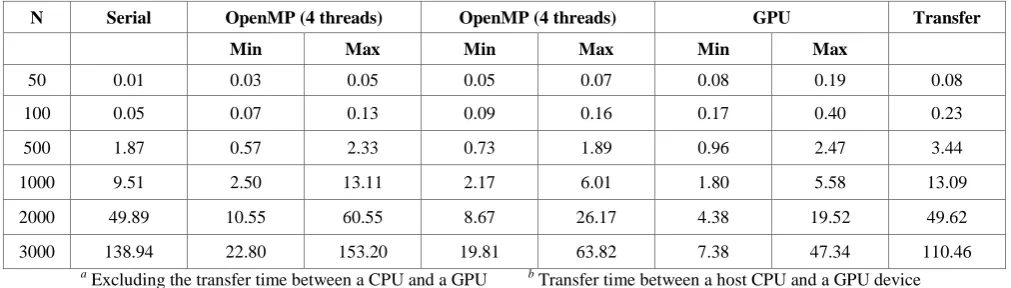
Since it is not easy to choose CUDA or OpenMP on the parts suitable to shared memory parallelism, we performed a simple test to compare CUDA and OpenMP. Devices normalized ‒ divided every element of a vector by its norm ‒ n vectors which consist of n elements. Parallelization decomposes this algorithm into n thread operations. We utilized two Intel Xeon E5606 2.13GHz quad-core CPUs and one NVIDIA Quadro 4000 GPU. OpenMP calculation used 4 or 8 CPU cores (i.e., 4 or 8 threads), while CUDA calculation used 1 GPU device with 256 cores. Table II shows how computation time changes as the number n increases. CUDA calculation looks faster when n exceeds 1000. On the other hand, the minima of OpenMP are always less than the maxima of CUDA because the speed of OpenMP or CUDA depends on the way of memory access. Moreover, the parallelization with CUDA spends much more time whenever transferring between a GPU device and a CPU host.

Looking into the test result (Table 2) and Table 1, we extracted some guidelines for choice of shared memory parallelization methods. It looks difficult even for faster CPUs to prevail over GPUs when n exceeds 1000, and it should be considered that Quadro 4000 is not that fast in comparison with other GPUs of compute capability 2.x [22]. In

consideration of large-scale calculations, since small-scale calculations do not need hybrid parallelization, CUDA should be preferred in most cases where coalesced memory access [23] is possible and the amount of data transferred between GPU and host is small compared to the calculation time of the data. Otherwise, OpenMP should be chosen because its memory access requires locality [24-29], as opposed to coalesced memory access. However, if either the GPU (CUDA) or CPU (OpenMP or serial) parts continue too long, CPUs can take over a small portion of the CUDA-favored part or vice versa because GPUs can operate independently of CPUs.

One can apply these rules to every part of DFT procedure, specifically. Since each term in the effective potential can be calculated independently, one can apply CUDA and OpenMP alternately in the effective potential part, i.e., CUDA for the first term and OpenMP for the second term and so on. On the other hand, the choice is not trivial for the density calculation part, but one can try dynamic load balancing between CUDA and OpenMP like Brown et al. [30]. It is also difficult to settle the general choice for the diagonalization computations because the choice should depend on its diagonalizing method, but we can obtain a hint from the fact that this part is full of matrix manipulation. CUDA should be chosen if parallelizable loops of basis function index are two-fold or more in cases like matrix multiplication. If such a parallelizable loop is just a single loop, the suitable shared memory parallelization method should be chosen to minimize data transfer between CPUs and GPUs, but it seems that CUDA should be preferred in most cases considering that DFT calculation scale will become larger and larger.

The above argument can be accompanied with MPI. MPI can intervene in CUDA or OpenMP sections, especially in a calculation of effective potential or densities where MPI can be idle. MPI can share loads with CUDA or OpenMP since the number of auxiliary basis functions is usually so large. Then the calculation of effective potential part will be filled with rotations of MPI+CUDA and MPI+OpenMP, but to take advantage of simultaneous work of GPUs and CPUs, their sequence should be

Step 1: CUDA calculation

Step 2: OpenMP calculation

Step 3: MPI communication of OpenMP results

Step 4: Transferring CUDA results from GPUs to their hosts

Table 2. Computation time (millisecond) for normalization of n vectors of n complex number elements (Average of 10 times). N Serial OpenMP (4 threads) OpenMP (4 threads) GPU Transfer

Min Max Min Max Min Max

50 0.01 0.03 0.05 0.05 0.07 0.08 0.19 0.08

100 0.05 0.07 0.13 0.09 0.16 0.17 0.40 0.23

500 1.87 0.57 2.33 0.73 1.89 0.96 2.47 3.44

1000 9.51 2.50 13.11 2.17 6.01 1.80 5.58 13.09

2000 49.89 10.55 60.55 8.67 26.17 4.38 19.52 49.62

3000 138.94 22.80 153.20 19.81 63.82 7.38 47.34 110.46

a

Excluding the transfer time between a CPU and a GPU b Transfer time between a host CPU and a GPU device

The strategy for conversion from the MPI+CUDA 2-way hybrid parallelization to the 3-way hybrid parallelization is straightforward. Looking into Tables 1 and 2, one can find that all OpenMP parts should convert into CUDA version unless data transfers between GPUs and CPUs are not severe.

If a data transfer is not negligible, the OpenMP part should return to its serial code form. The strategy for effective potential part in the above paragraph can be modified by changing the step 2 with CUDA and removing the step 3.

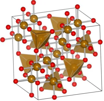
Fig 2: (Color online) 3D view [31] of cubic crystal stucture of our magnetite system

Table 3. Time sharing of typical 1 CPU DFT calculation on the magnetite system by OpenMX

Routine Time (seconds) Share (%)

Set OLP Kin 287.037 0.130

Set Nonlocal 872.376 0.394

Set Hamiltonian 7091.817 3.201

Poisson 3.429 0.002

Diagonalization 208811.550 94.236

Mixing DM 62.969 0.028

Force 1433.113 0.647

Total Energy 299.321 0.135

Set Aden Grid 2.011 0.001

Set Orbitals Grid 6.170 0.003 Set Density Grid 2705.252 1.221

Others 7.984 0.004

3.

APPLICATION TO OpenMX

These techniques were tested on OpenMX 3.6 code with a magnetite system. OpenMX [2,32,33] was developed for quantum simulations of nano-scale materials and can deal with large-scale calculations on parallel computers, by implementing MPI and OpenMP. Our magnetite system consists of 56 atoms (24 iron atoms and 32 oxygen atoms) in the calculation unit-cell (Fig. 2), and the atoms’ coordinates

and the unit-cell size were borrowed from X-ray measurement [34]. Total numbers of k-points, main basis functions and auxiliary basis functions used in this system are 64, 1040 and 512000, respectively. For this system, the authors performed spin-collinear band calculation within GGA.

Time consuming analysis of serial calculation of this system summarized in Table 3 reveals that the diagonalization part possesses the most of the CPU time up to 94 %. Therefore, it was beneficial to focus only on the diagonalization that solves the eigenvalue equations. In OpenMX, diagonalization within spin-collinear band calculation is governed by the routine called Band_DFT_Col, which consists of following parts (The first part belongs to the part of effective potential calculation, but Band DFT Col includes it in OpenMX).

Part 1: Giving k-point dependence to overlap matrix S and Hamiltonian H

Part 2: Diagonalizing S to rearrange S

Part 3: Multiplication of matrices to make S†HS

Part 4: Diagnoalizing S†HS to get eigenvalues or eigenvectors

Part 5: Finding chemical potential and calculating band energy.

Part 6: Calculating charge density matrix and energy density matrix

Then the algorithm of Band_DFT_Col is, crudely expressed,

for (assigned k-points) {

Part 1 Part 2 Part 3

Part 4 (obtaining eigenvalues) }

Part 5

for (assigned k-points) {

Part 1 Part 2 Part 3

Part 4 (obtaining eigenvectors) }

Part 6

The parts 2 and 4 use the Householder algorithm for tridiagonalization [35] and a LAPACK [36] routine among dstevx, dstedc or dstegr. The parts 3 and 4 use ZGEMM routine in LAPACK [36]. The parts 1, 5 and 6 are just multiplications and summations. Table 4 exhibits time sharing of each part for single CPU calculation.

(OpenMP or serial) CPU code treats Hamiltonian H, but exchanging S and H is possible between the CPU code and the CUDA code. The part 5 does not need parallelization because time sharing is very small. CUDA has advantages also in the part 6 because the main multi loop of this part can be converted into a large loop of O(n2) where n is the number of basis functions.

Table 4. Percentage of the routines to consume serial calculation CPU time in Band_DFT_Col.

Routine Share (%)

Imposing k dep. (Part 1) 0.224 Diagonalizing S (Part 2) 39.531

Making S†HS (Part 3) 15.023 Diagonalizing S†HS (Part 4) 39.390 Chem. Pot. & Band E. (Part 5) 0.001

Density Matrix (Part 6) 5.788

Sum 99.956

The parts 2 and 4 actually call the same subroutine named Eigen_HH, composed of four steps: the Householder process, calling a LAPACK routine (dstevx, dstegr or dstedc), rearrangement of eigenvectors, and normalization. The last two steps are activated only given an option demanding eigenvectors, and CUDA was chosen for them because each of them has only one parallelizable loop but the amount of data transfers does not depend on whether CUDA or OpenMP is used. Later, a test verified that CUDA is appropriate for them in case of calculating our magnetite system with 1040 basis functions.1 The LAPACK routines, dstevx, dstegr and dstedc, could not be parallelized, but a small portion of the step rearranging eigenvectors can be calculated on GPUs while a LAPACK routine is working on CPUs.

The remaining first step, tridiagonalization by Householder algorithm [35], is an iterative loop that consists of following procedures [2,38]. For the ith iteration (i = 1, 2, … , n-1. n: rank of the input matrix), where B is the matrix obtained from (i-1)th iteration (initially the input matrix),

Procedure 1: Setting the vector u as ith column vector of B

Procedure 2: Calculating the scalar s (norm of the above vector u) and change the ith element of u by subtracting s.

Procedure 3: Storing the ith elements of a few vectors to be used in the rearrangement of eigenvectors

Procedure 4: Calculating the vector p′ (= B ∙ u / (2u2) ) and the dot product of p′ and u

Procedure 5: Calculating the vector q′ from p′ and p′ ∙ u. (See reference [38] for the definition of q′)

Procedure 6: Partial transformation of B by subtracting a matrix composed of0020products of the u and q′ elements. (See reference [38] for the form of the subtracting matrix)

The main loop of the Householder process in Eigen_HH is repeating above procedures until the target matrix becomes a real symmetric tridiagonal matrix. As our policy for matrix

manipulation, we applied CUDA to procedure 6 which has a double parallelizable loop of basis function index. The procedure 3, containing no loop, naturally remained not parallelized. Single parallelizable loops were found in procedures 1, 2, 4, and 5, but CUDA was applied to 1, 4, and 5. Due to the procedure 6, CUDA was the inevitable choice in the procedures 1 and 5 to avoid data transfer between CPUs and GPUs. The procedure 2 and 4 includes summation, which leads to inefficiency in parallelization, but the procedure 4 can be performed in GPUs during the procedure 3. (Dot product calculation consists of multiplication and addition. It was found that addition in dot product calculation is more efficient on CPUs even considering data transfer between CPUs and GPUs. So the addition in the procedure 4 was assigned to CPUs.) So the only procedure 2 should be converted by OpenMP or should remain the serial form.

After applying our strategies, it was found that OpenMP fraction would be so small. In our modified Band_DFT_Col, OpenMP was used in some initial settings, data type conversion of matrices, and the procedure 2 in Eigen_HH. All these occupy tiny portions of the whole Band_DFT_Col, which suggests that MPI+CUDA parallelization should reduce computational time much more than 3-way hybrid parallelization. Accidentally, these OpenMP parts are disadvantageous to be converted by CUDA. So MPI+CUDA 2-way parallelization is possible without CUDA conversion of these parts.

Even under our hybrid politics, comparing parallelizable fractions shows that OpenMX 3.6 DFT code prefers MPI to other parallelization methods. MPI parallelized 99.5 %, close to 100 %, of the CPU single core time of Band_DFT_Col mainly by parallelization on k-points. CUDA and OpenMP parallelized 88.2 % of the CPU single core time. Although it is difficult to distinguish OpenMP time and CUDA time completely due to GPUs’ ability of independent working, CUDA parallelizable fraction can be approximated as 88 % from our OpenMP time measurement close to 0.2 %, but 88 % is about 12 % different from that of MPI. According to Amdahl’s law, if computation power is four times of CPU single core’s, the result speedup by MPI will be about 3.9 while that by CUDA will be about 2.9. In order to prevail over a quad-core CPU with MPI, a GPU with CUDA may need computational power more than about 6.5 times of CPU single core’s.

The machine setup is a single computer with two Intel Xeon E5606 processors and two NVIDIA Quadro 4000 graphics cards. The main board of the machine has: two Intel Xeon E5606, each with 4 cores at 2.13Ghz, each and 12GB of DDR3 system memory that allows for a theoretical 17.06 GFLOPS performance in single core double precision floating point calculation [39]. The memory test for Xeon E5606 single core was done by STREAM 5.10, and we obtained 6.48 GB/s as bandwidth. Each of the two NVidia Quadro 4000 GPU processors has 256 cores and 2GB of GDDR5 memory with 89.6 GB/s bandwidth [40]. The peak performance for one of our GPUs is 243.2 GFLOPS using double precision numbers [40]. It is important to note that these are peak theoretical performances if all computations are performed with no latency or empty processing cycles.

references to estimate the efficiency of CUDA parallelization because the ideal speedup calculation was based on theoretical peak performances and a theoretical bandwidth although CPU memory bandwidth is real one.

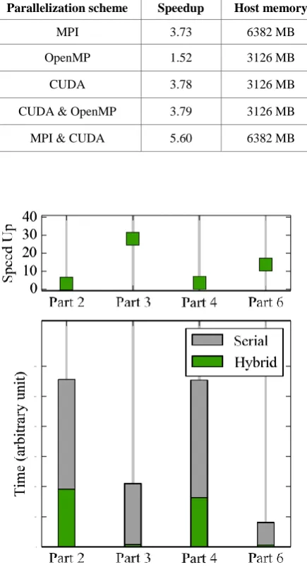
Table 5. Speedup of Band_DFT_Col by each parallelization scheme using 1 quad-core CPU and 1 GPU,

compared to serial calculation, and CPU memory usage. Parallelization scheme Speedup Host memory

MPI 3.73 6382 MB

OpenMP 1.52 3126 MB

CUDA 3.78 3126 MB

CUDA & OpenMP 3.79 3126 MB

MPI & CUDA 5.60 6382 MB

Fig 3: (Color online) Time and speedup for the principal parts of Band_DFT_Col, by 1 CPU and 1 GPU within OpenMP+CUDA parallelization (denoted Hybrid).

The experiment first used one quad-core CPU and one GPU, and the result is summarized in Table 5. Since MPI parallelizes the code with respect to k-points, in case of MPI+CUDA parallelization, more k-points were allocated to GPUs, applying a weighting ratio of four, from the speedup by one GPU and one CPU core, denoted CUDA in Table 5. Consequently, the best speedup was obtained by MPI+CUDA parallelization. Although OpenMP’s memory cost is about two times lower than MPI, it stands the worst in speedup, maybe due to memory bottleneck, low parallelizable fraction or cache miss. CUDA enhances OpenMP’s speedup well. However, the speedups by CUDA do not reach our expectation. Considering that Quadro 4000 is not that fast among compute capability 2.x [22] GPUs, larger speedups can be expected on other GPUs.

The respective routines were closely examined to find reasons of CUDA parallelization’s unsatisfactory efficiency. As shown by Fig. 3, parts 2 and 4 (diagnoalizing S and S†HS) are obstacles in increasing the whole speed. The strangely high speedup of part 3 (making S†HS), mostly consisting of calling ZGEMM, implies that ZGEMM fits CUDA parallelization although the speedup over 14 seems to be caused by elimination of code lines unnecessary to CUDA parallelization. ZGEMM shows the highest GPU speedup in Maintz et al.’s result as well [8]. ZGEMM appears to be also the reason why part 4 (calling Eigen_HH and ZGEMM each once) gains higher speedup than part 2. Therefore, Eigen_HH routine was suspected to be the main obstacle.

Table 6. Percentage of the partial routines to consume serial calculation CPU time in Eigen HH and speedups in

each routine by 1 GPU + OpenMP (4 threads) parallelization.

Routine Percentage Speedup

Householder tridiagonalization 43.17 % 5.23

LAPACK routine 14.75 % 1.00

Rearrangement of eigenvectors 42.02 % 4.23 Normalization & transpose 0.07 % 1.84

Table 7. Speedup of Band_DFT_Col by each parallelization scheme using 2 quad-core CPUs and 2 GPUs, compared to serial calculation, and CPU memory usage as well as speed increase rate by processor doubling, i.e., by adding 1 CPU and 1 GPU. OpenMP used 4 threads

in each MPI process. Parallelization

scheme Speedup Host memory

Increase rate

MPI 6.33 10683 MB 70 %

MPI & OpenMP 2.89 4211 MB 90 %

3-way hybrid 7.55 4211 MB 99 %

MPI & CUDA 10.94 10683 MB 95 %

Thus the performance time of Eigen_HH was analyzed (Table 6). Among the four steps of Eigen_HH, the tridiagonalization and rearrangement of eigenvectors occupy about 85 % of the single CPU core calculation time of Eigen_HH, and their speedups by 1 GPU and 1 quad-core CPU were measured to be 5.23 and 4.23, respectively within CUDA+OpenMP parallelization. Householder algorithm seems to be optimized to serial calculation, which appears to be the reason for the tridiagonalization’s low speedup. The low efficiency of the rearranging eigenvectors is naturally expected since it has only single parallelizable loops. The LAPACK routine also seems the reason why the speedups of part 2 and 4 are less than four. In any case, further speed increase needs a considerable change of algorithm, but that is beyond the scope of this paper.

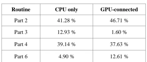
enhancement by CUDA is slightly more effective than the 1 CPU and 1 GPU cases. Accuracy of these hybrid schemes is very similar to the non-CUDA cases since these hybrid schemes do not change the essence of the code’s algorithm. A process-wise analysis can reveal room of enhancement. In case of the MPI & CUDA, we assigned k-points to MPI processes asymmetrically, giving four times heavier weight to a GPU-connected process compared with a CPU only process. The result speedup of each MPI process ranges from 10.9 to 11.9, showing not bad weight balance. The quadruple weight to GPU-connected processes does not look like the reason of the 1.0 range because the speedups of the GPU-connected processes were found to be 11.3 and 11.4. The time sharing of the slowest CPU only process (Table 8) is close to Table 4 since only k-point division increase the speed of CPU only processes. The time sharing of GPU-connected processes is related to the previous analyses (Fig 3 and Table 6). If Eigen_HH is edited to get 20 % speed increase, more weight can be given to GPU-connected processes and get a speedup of Band_DFT_Col close to 12. The analysis of 3-way hybrid case (not shown here) is similar to the CUDA & OpenMP case as indicated by the 99 % increase rate in Table 7 because the assignment of k-points is symmetric. Thus Fig 3 and Table 6 hold for the 3-way hybrid, just doubling the speedups. The Eigen_HH affects more in this case, and the 20 % speed increase of the Eigen_HH can result in a speedup close to 9 within the 3-way hybrid scheme.

Table 8. Time sharing percentage of the principal parts of Band_DFT_Col in the slowest CPU only process and the

slowest GPU-connected process in the MPI & CUDA scheme in Table 7.

Routine CPU only GPU-connected

Part 2 41.28 % 46.71 %

Part 3 12.93 % 1.60 %

Part 4 39.14 % 37.63 %

Part 6 4.90 % 12.61 %

In spite of lack of great change of the whole algorithm, the highlight of these hybrid schemes is that efficiency hardly drops as processors added. By comparison of the 2 CPUs and 2 GPUs cases to the 1 CPU and 1 GPU cases (MPI to MPI, OpenMP to MPI+OpenMP, CUDA+OpenMP to 3-way hybrid, and MPI+CUDA to MPI+CUDA), the speed increase rates for the cases including CUDA are superior to the non-CUDA cases. Each GPU is independent and interacts with the whole system only by its PCI-Express bus, which compensates the main memory bottleneck effect due to competition among CPU cores. In MPI+CUDA scheme, one CPU core’s different action may further compensate the bottleneck effect.

These results reveal two features of hybrid parallelization with CUDA without changing the essence of the code’s algorithm. Large speedup enhancement in the cases with OpenMP suggests that GPUs’ aid to parallelization is very useful to huge memory consuming calculation where few MPI processes per node are available. Little efficiency drop by processor addition implies the hybrid parallelization will be necessary to many multi-core CPU systems where adding CPUs will trigger large efficiency drop. From both points, it is shown that even easy conversion with CUDA will be more

or less helpful to DFT calculation on parallel computing systems.

4.

CONCLUSIONS

The authors applied hybrid parallelization including CUDA to a MPI-friendly DFT source code, originally not optimized to CUDA. Two types of hybridization are possible such as 3-way hybrid scheme saving memory with equally divided load and 2-way hybrid scheme maximizing speed by weighting of unequal loads. The authors established several rules in editing NAO DFT codes to parallelize with hybrid schemes, by analyzing NAO DFT codes’ property and comparing OpenMP and CUDA on a simple test. Applying these rules is easy because they do not change the essence of the codes’ algorithm.

The test was performed on a magnetite material system with OpenMX 3.6 code by utilizing a hardware system containing 2 Xeon E5606 CPUs and 2 Quadro 4000 GPUs. 3-way hybrid scheme obtained the speedup of 7.55 and saved nearly 60 % of memory. 2-way hybrid scheme obtained the speedup of 10.94. CUDA did not reach our expectation, due to the relatively low CUDA parallelizable fraction of the code and its algorithm’s inefficiency for CUDA, compared with MPI. Nevertheless, CUDA capable GPUs complement the efficiency of OpenMP and compensate the CPUs’ excessive competition for memory in MPI.

GPGPU appears meaningful even by simple conversion within hybrid parallelization with a not-so-fast GPU. Note that we assumed compute capability 2.x [22], and a change of GPU can give better performance because the Quadro 4000 is only a midrange GPU when compared with the NVIDA Tesla’s. If one wants to further speed up the code and has a strong will to meticulously edit the code, one can change the essential algorithms of a DFT code not immediately CUDA-friendly.

5.

ACKNOWLEDGMENTS

We thank Prof. T. Ozaki for allowing us to edit OpenMX 3.6 code. This work was supported by the Technology Innovation Program (10036459, Development of center to support QoLT industry and infrastructures) funded by the MOTIE/KEIT and the National Research Foundation of Korea (NRF) grant funded by the Korea government (MEST. No. 2009-0092790).

6.

REFERENCES

[1] A. Ghosh, P.R. Taylor, "High-level ab initio calculations on the energetic of low-lying spin states of biologically relevant transition metal complexes: a first progress report", Curr. Opin. Chem. Biol. 7:113‒124 2003. [2] OpenMX webpage, http://www.openmx-square.org/ [3] SIESTA webpage, http://www.icmab.es/siesta/

[4] Message Passing Interface Forum, http://www.mpi-forum.org/

[5] OpenMP, http://openmp.org/wp/

[6] H. Jin, D. Jespersen, P. Mehrotra, R. Biswas, L. Huang, B. Chapman, "High performance computing using MPI and OpenMP on multi-core parallel systems", Parallel Comput. 37:562‒575, 2011.

[8] S. Maintz, B. Eck, R. Dronskowski, "Speeding up plane-wave electronic-structure calculations using graphics-process units", Comput. Phys. Commun. 182:1421‒1427, 2011.

[9] K.A. Wilkson, P. Sherwood, M.F. Guest, K.J. Naidoo, "Acceleration of the GAMESS-UK Electronic Structure Package on Graphical Processing Units", J. Comput. Chem. 32(10):2313‒2318, 2011.

[10] L. Genovese, M. Ospici, T. Deutsch, J.-F. Méhaut, A. Neelov, S. Goedecker, "Density functional theory calculation on many-cores hybrid central processing unit-graphic processing unit architectures", J. Chem. Phys. 131:034103, 2009.

[11] C.T. Yang, C.L. Huang, C.F. Lin, "Hybrid CUDA, OpenMP, and MPI parallel programming on multicore GPU clusters", Comput. Phys. Commun. 182:266‒269, 2011.

[12] F. Wang, C.-Q. Yang, Y.-F. Du, J. Chen, H.-Z. Yi, W.-X. Xu, "Optimizing linpack benchmark on GPU-accelerated petascale supercomputer", J. Comput. Sci. & Technol. 26(5): 854‒865, 2011.

[13] H.-Y. Schive, U.-H. Zhang, T. Chiueh, "Directionally unsplit hydrodynamic schemes with hybrid MPI/OpenMP/GPU parallelization in AMR", Int. J. High Perform. C. 26(4):367‒377, 2011.

[14] F. Lu, J. Song, F. Yin, X. Zhu, "Performance evaluation of hybrid programming patterns for large CPU/GPU heterogeneous clusters", Comput. Phys. Commun. 183:1172‒1181, 2012.

[15] F. Lu, J. Song, X. Cao, X. Zhu, "CPU/GPU computing for long-wave radiation physics on large GPU clusters", Comput. Geosci. 41:47‒55, 2012.

[16] C.T. Hsu, K.F. Sin, S.W. Chiang, "Parallel computation for Boltzmann equation simulation with Dynamic Discrete Ordinate Method (DDOM)", Comput. Fluids 54:39‒44, 2012.

[17] M.H. Fadhil, M.I. Younis, "Parallelizing RSA Algorithm on Multicore CPU and GPU", Int. J. Comput. Appl. 87(6):15‒22, 2014.

[18] You can see our patch for OpenMX3.6 at http://www.eriksevre.com/projects/openmxcuda/ [19] Martin R.M. 2004 Electronic Structure: basic theory and

practical methods. Cambridge University press.

[20] Kohanoff J. 2006 Electronic Structure Calculations for Solids and Molecules. Cambridge University press. [21] U. von Barth, L. Hedin, "A local exchange-correlation

potential for the spin polarized case: I", J. Phys. C: Solid State Phys. 5:1629‒1642, 1972.

[22] CUDA C programming Guide,

http://docs.nvidia.com/cuda/cuda-c-programming-guide/ [23] CUDA C Best Practices Guide,

http://docs.nvidia.com/cuda/cuda-c-best-practices-guide/

[24] D. Hisley, G. Agrawal, P. Satya-narayana, L. Pollock, "Porting and performance evaluation of irregular codes using OpenMP", Concurrency: Pract. Exper. 12:1241– 1259, 2000.

[25] B. Chapman, F. Bregier, A. Patil, A. Prabhakar, "Achieving performance under OpenMP on ccNUMA and software distributed shared memory systems", Concurrency Computat.: Pract. Exper. 14:713–739, 2002.

[26] A. Marowka, Z. Liu, B. Chapman, "OpenMP-oriented applications for distributed shared memory architectures", Concurrency Computat.: Pract. Exper. 16:371–384, 2004.

[27] M.J. Berger, M.J. Aftosmis, D.D. Marshall, S.M. Murman, "Performance of a newCFD flowsolver using a hybrid programming paradigm", J. Parallel Distr. Com. 65:414423, 2005.

[28] F. Broquedis, N. Furmento, B. Goglin, P.-A. Wacrenier, R. Namyst, "ForestGOMP: An Efficient OpenMP Environment for NUMA Architectures", Int. J. Parallel Prog. 38:418–439, 2010.

[29] A. Marongiu, L. Benini, "An OpenMP Compiler for Efficient Use of Distributed Scratchpad Memory in MPSoCs", IEEE T. Compu. 61(2):222–236, 2012. [30] W.M. Brown, P. Wang, S.J. Plimpton, A.M. Tharrington,

"Implementing molecular dynamics on hybrid high performance computers – short range forces", Comput. Phys. Commun. 182:898–911, 2011.

[31] K. Momma, F. Izumi, "VESTA: a three-dimensional visualization system for electronic and structural analysis", J. Appl. Crystallogr., 41:653–658, 2008. [32] T. Ozaki, H. Kino, "Numerical atomic basis orbitals from

H to Kr", Phys. Rev. B 69:195113, 2004.

[33] T. Ozaki, H. Kino, "Efficient projector expansion for the ab initio LCAO method", Phys. Rev. B 72:045121, 2005. [34] H.C. Hamilton, "Neutron Diffraction Investigation of the 119°K Transition in Magnetite", Phys. Rev. 110(5):1050–1057, 1958.

[35] A.S. Householder, "Unitary Triangularization of a Nonsymmetric Matrix", J. ACM 5(4):339–342, 1958. [36] Netlib website, http://www.netlib.org/

[37] CUBLAS website, http://developer.nvidia.com/cublas [38] OpenMX technical note: Householder Method for

Tridiagonalization, http://www.openmx-square.org/tech_notes/tech10-1_0.pdf

[39] Intel Xeon 5600 series information website, http://download.intel.com/support/processors/xeon/sb/xe on 5600.pdf

[40] NVIDIA QUADRO 4000 website,