New Procedure of Finding an Initial Basic Feasible Solution of the Time Minimizing Transportation Problems

http://dx.doi.org/10.4236/ojapps.2015.510062

New Procedure of Finding an Initial Basic

Feasible Solution of the Time Minimizing

Transportation Problems

Mollah Mesbahuddin Ahmed1_{, Md. Amirul Islam}1_{, Momotaz Katun}2_{, Sabiha Yesmin}1_,

Md. Sharif Uddin1

1_{Department of Mathematics, Jahangirnagar University, Savar, Dhaka, Bangladesh} 2_{Department of Mathematics, Bangladesh University, Dhaka, Bangladesh}

Email: [email protected], [email protected], [email protected], [email protected], [email protected]

Received 28 September 2015; accepted 26 October 2015; published 29 October 2015

Copyright © 2015 by authors and Scientific Research Publishing Inc.

This work is licensed under the Creative Commons Attribution International License (CC BY). http://creativecommons.org/licenses/by/4.0/

Abstract

Minimization of transportation time is a great concern of the transportation problems like the cost minimizing transportation problems. In this writing, a transportation algorithm is devel-oped and applied to obtain an Initial Basic Feasible Solution (IBFS) of transportation problems in minimizing transportation time. The developed method has also been illustrated numerically to test the efficiency of the method where it is observed that the proposed method yields a bet-ter result.

Keywords

Transportation Problem, Initial Basic Feasible Solution, Minimizing, Transportation Time

1. Introduction

A special class of Linear Programming Problem is transportation problem, where the main objective is to mi-nimize the cost of distributing a product from a number of sources to a number of destinations. This type of problem is known as cost minimizing transportation problem. The problem of minimizing transportation cost has been studied since long and is well known by [1]-[15].

short storage period, where the speed of delivery is more important than the transportation cost. This type of transportation problem is known as time minimizing transportation problem where the objective is to minimize the transporting time rather than the cost of transportation.

An initial basic feasible solution for minimizing the time of transportation can be obtained by using any well known methods such as, North West Corner Method (NWCM), Least Cost Method (LCM), Vogel’s Approxi-mation Method (VAM) and Extremum Difference Method (EDM). The time minimizing transportation problem had also been studied by a good number of researchers [16]-[20] and they introduced various algorithms for solving time minimizing transportation problems. Garfinkel and Rao in 1971 solved time minimizing transporta-tion problems [21]. Hammer [16] and Szwarc [22] used labeling techniques to solve such kind of problems re-spectively in 1969 and 1971. In [23], Nikolic proposed an algorithm to obtain the minimum of the total trans-portation time. Very recently M. Sharif Uddin [18] has developed an efficient technique of minimizing the time of a transportation problem.

2. Proposed Procedure of Finding an Initial Basic Feasible Solution

It is considered that the readers are well acquainted with transportation problem. Basing on this consideration, a new procedure of finding an initial basic feasible solution of the time minimizing transportation problems is been illustrated below:

 Step-1: Identify the Largest Element (LE) of every row and every column in the transportation table and write down them in outer column of the supply and lower row of the demand.

 Step-2: Determine the magnitude of the difference of row largest element and column largest element cor-responding to each element.

 Step-3: Place the value obtained in step-2 on the right bottom of the corresponding elements.

 Step-4: Place the Row Distribution Indicators (RDI) and the Column Distribution Indicators (CDI) just after and below the supply limits and demand requirements respectively within first bracket, which are the differ-ence of the largest and nearest-to-largest (Second largest) of right bottom entries. If there are two or more largest entries, the RDI or CDI is to be considered as zero.

 Step-5: Identify the largest number among the RDI and CDI in each level. Choose the smallest time unit along the highest RDI or CDI. If there are two or more number of highest RDI or CDI; choose that highest indicator along which the smallest time element is present. If there are two or more number of smallest time element, choose any one of those arbitrarily.

 Step-6: Allocate minimum of supply/demand values on the left top of the corresponding smallest time unit selected in Step-5.

 Step-7: Check whether exactly one of the row/column corresponding to the selected cell has zero supply/ zero demand, respectively. If so, delete the row/column which has the zero supply/zero demand. Again if it is found that both the supply and demand has become zero corresponding to the selected cell, delete either the row or column but not both.

 Step-8: Match the supply/demand of the left out row/column with the remaining demands/supplies of the undeleted columns/row.

 Step-9: Repeat Step: 4 to 6 until all the rim requirements are satisfied.

 Step-10: Determine the largest time Tk corresponding to basic cells.

3. Algorithm for Optimality Test

Algorithm for finding the optimal time for time minimization transportation problems are described below:

 Step-1: Determine an initial basic feasible solution using above method.

 Step-2: Determine the largest time Tk corresponding to the basic cells and cross off all non-basic cellstij≥Tj.  Step-3: Construct a loop for the basic cells corresponding to largest time Tk including a non-basic cell in such a way that the allotment in the cell with Tk can be shifted to the non-basic cell in the loop by readjust-ment of row and column sum, the value at Tk cell is zero and no variables becomes zero or negative. If no such loop can be formed, the solution under test is optimum. Otherwise move to the next step.

4. Illustrative Example

4.1. Example-1

Table 1shows the time required to shift a load from origins to destinations. It is required to find the optimum plan for shipment to minimize the time of shipment.

Table 1. Data of the example-1.

Origins Destinations Supply

D1 D2 D3

O1 13 21 14 13

O2 8 12 21 20

O3 15 17 19 5

Demand 12 15 11

4.1.1. Initial Basic Feasible Solution

From the above table it is seen that total supply and total demand are equal. Hence the given transportation problem is a balanced one. Obtaining IBFS for Example-1 using the Proposed Algorithm is shown in Table 2.

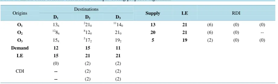
Table 2.Initial basic feasible solution of example-1using proposed algorithm.

Origins Destinations Supply LE RDI

D1 D2 D3

O1 136 2₂₁₀ 11₁₄₀

13 21 (6) (0) (0)

O2 1286 8_{120 210}

20 21 (6) (0) --

O3 154 5_{172 192}

5 19 (2) (0) (0)

Demand 12 15 11

LE 15 21 21

CDI

(0) (2) (2)

-- (2) (2)

-- (2) (2)

We see that the number of basic variables is 5 = (3 + 3 − 1) and the set of basic cells do not contain a loop. Thus the solution obtained is a basic feasible solution and the initial basic feasible solution is x12 = 2, x13 = 11,

x21 = 12, x22 = 8, x32 = 5 and the shipping time of basic cells are t12 = 21, t13 = 14, t21 = 8, t22 = 12, t32 = 17.

Therefore, in order to complete the shifting it takes the time T1 = max{t12, t13, t21, t22, t32} = max{21, 14, 8, 12,

17}= 21 units of time.

4.1.2. Optimality Test

 Iteration-1: From the IBFS, it is found that the largest time is T1 = 21, therefore we cross off the non-basic

cell (2, 3) which contains equal time unit to T1. Let us construct a loop for the basic cells corresponding to

the largest time T1 = 21 including the non-basic cell (1, 1) which is called entering cell. The constructed loop

in this iteration is shown in Table 3.

Table 3. Consturucted loop in iteration-1.

Origins Destinations Supply

D1 D2 D3

O1 13 ₊

2₂₁

− 1114 13

O2

12₈ −

8₁₂

+ 21 20

O3 15 5_{17 19 5}

The allocation is readjusted in the corner of the loop and a new solution is obtained which is shown in Table 4.

Table 4.Readjusted allocation in iteration-1.

Origins Destinations Supply

D1 D2 D3

O1 213 21 1114 13

O2 10₈ 10_{12 21 20}

O3 15 5_{17 19 5}

Demand 12 15 11

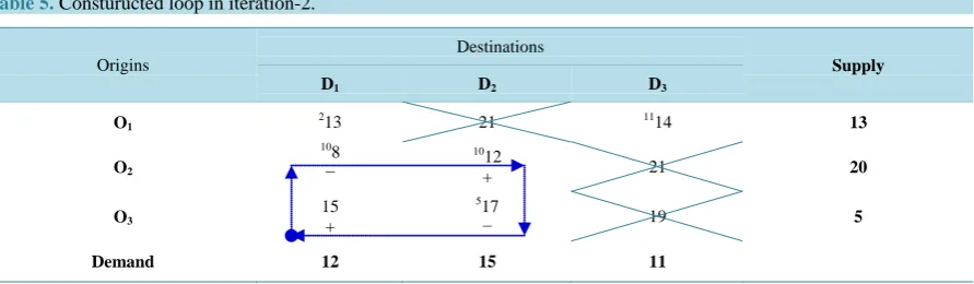
 Iteration-2: Now largest time is T2 = 17, therefore we cross off the cells (1, 2) and (3, 3) which contain larger

time units than T2. Let us construct a loop for the basic cells corresponding to the largest time T2 = 17

in-cluding the non-basic cell (3, 1). The constructed loop in this iteration is shown in Table 5.

Table 5. Consturucted loop in iteration-2.

Origins

Destinations

Supply

D1 D2 D3

O1 213 21 11₁₄

13

O2

10₈ −

10₁₂

+ 21 20

O3 15

+

5₁₇

− 19 5

Demand 12 15 11

Readjust the allocation in the corner of the loop, we obtain a new solution which is shown in Table 6.

Table 6. Readjusted allocation in iteration-2.

Origins Destinations Supply

D1 D2 D3

O1 2_{13 21} 11_{14 13}

O2 58 15_{12 21}

20

O3 515 17 19 5

Demand 12 15 11

 Iteration-3: Now largest time is T3 = 15, therefore the cell (3, 2) which contains larger time unit than T3 is

crossed off. Now all the crossed off cells including the crossed off cell in this stage is shown in Table 7.

Table 7. All the crossed off cells.

Origins

Destinations

Supply

D1 D2 D3

O1 213 21 11₁₄

13

O2 5₈ 15_{12 21 20}

O3 5_{15 17 19 5}

Now no loop can be formed originating from the cell (3, 1). Thus the obtained solution x11 = 2, x13 = 11, x21 =

5, x22 = 15, x31 = 5 is optimum and the optimum shipment time is max {13, 14, 8, 12, 15} = 15 time units.

4.2. Example-2

Some equipment is to be transported from three origins to three destinations. The supply at the origins, the de-mand at the destinations and the time of shipment are shown in Table 8.

Table 8. Data of the example-2.

Origins Destinations Supply

D1 D2 D3

O1 15 7 25 12

O2 8 12 14 17

O3 17 19 21 7

Demand 12 10 14

It is required to find the optimum plan for shipment to minimize the total time of shipment.

4.2.1. Initial Basic Feasible Solution

From Table 8, it is seen that total supply and total demand are equal. Hence the given transportation problem is a balanced one. Obtaining IBFS for Example-2 using the Proposed Algorithm is shown in Table 9.

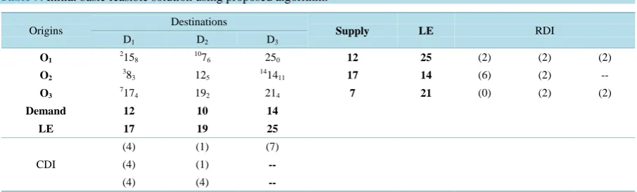
Table 9. Initial basic feasible solution using proposed algorithm.

Origins Destinations Supply LE RDI

D1 D2 D3

O1 2158 10_{76 250}

12 25 (2) (2) (2)

O2 383 125 14₁₄₁₁

17 14 (6) (2) --

O3 7174 192 214 7 21 (0) (2) (2)

Demand 12 10 14

LE 17 19 25

CDI

(4) (1) (7)

(4) (1) --

(4) (4) --

It is seen that the number of basic variables is 5 (=3 + 3 − 1) and the set of basic cells do not contain a loop. Thus the solution obtained is a basic feasible solution and the initial basic feasible solution is x11 = 2, x12 = 10,

x21 = 3, x23 = 14, x31 = 7 and the shipping time of basic cells are t11= 15, t12 = 7, t21= 8, t23 = 14, t31 = 17.

Therefore, in order to complete the shipment, it takes the time T1 = max{t11, t12, t21, t23, t31} = max{15, 7, 8, 14,

17} = 17 units of time.

4.2.2. Optimality Test

 Iteration-1: Now largest time is T1 = 17, therefore the non basic cells, (1, 3), (3, 2) and (3, 3) containing

larger time units than T1 are crossed off. These crossed off cells are shown in Table 10.

Table 10. All the crossed off cells.

Origins Destinations Supply

D1 D2 D3

O1 215 10_{7 25}

12

O2 38 12 14₁₄

17

O3 717 19 21 7

Now no loop can be formed originating from the cell (3, 1). Thus the obtained solution x11 = 2, x12 = 10, x21 =

3, x23 = 14, x31 = 7 is optimum and the optimum shipment time is max {15, 7, 8, 14, 17} = 17 units of time.

5. Comparative Study of the Results

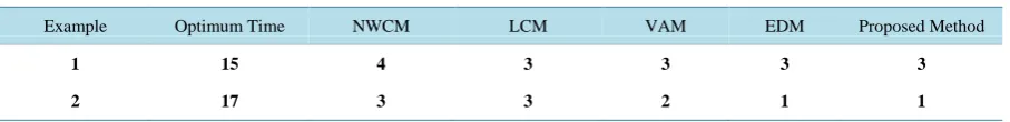
After obtaining an IBFS by the proposed method, the obtained result is compared with the solution obtained by other existing methods that how many number of iterations are to be required to obtain an optimum solution. This is shown in Table 11.

Table 11. Numer of iterations required to obtain optimum time.

Example Optimum Time NWCM LCM VAM EDM Proposed Method

1 15 4 3 3 3 3

2 17 3 3 2 1 1

6. Conclusion

In this writing, an algorithm has been discussed to solve time minimizing transportation problems. Efficiency of the developed algorithm is also been justified by solving numerical problems. During this process, a compara-tive study among the proposed method and the other existing methods is also carried out; where it is observed that the proposed method requires minimum number of iterations to obtain the optimal transportation time. Therefore, the proposed algorithm claims its wide application in the field of optimization in solving the time mi-nimizing transportation problem.

References

[1] Khan, A.R. (2011) A Resolution of the Transportation Problem: An Algorithmic Approach. Jahangirnagar University Journal of Science, 34, 49-62.

[2] Khan, A.R. (2012) Analysis and Resolution of the Transportation Problem: An Algorithmic Approach, M.Phil. Thesis, Department of Mathematics, Jahangirnagar University, Savar.

[3] Khan, A.R., Vilcu, A., Sultana, N. and Ahmed, S.S. (2015) Determination of Initial Basic Feasible Solution of a Transportation Problem: A TOCM-SUM Approach. Buletinul Institutului Politehnic Din Iasi, Romania, Secţia Auto-matica si Calculatoare, LXI (LXV), 1, 39-49.

[4] Khan, A.R., Banerjee, A., Sultana, N. and Islam, M.N. (2015) Solution Analysis of a Transportation Problem: A Com-parative Study of Different Algorithms. Bulletin of the Polytechnic Institute of Iasi, Romania, Section Textile, Lea-thership, in Press.

[5] Uddin, M.S., Anam, S., Rashid, A. and Khan, A.R. (2011) Minimization of Transportation Cost by Developing an Ef-ficient Network Model. Jahangirnagar Journal of Mathematics & Mathematical Sciences, 26, 123-130.

[6] Islam, Md.A., Khan, A.R., Uddin, M.S. and Male, M.A. (2012) Determination of Basic Feasible Solution of Transpor-tation Problem: A New Approach. Jahangirnagar University Journal of Science, 35, 101-108.

[7] Islam, Md.A., Haque, Md.M. and Uddin, Md.S. (2012) Extremum Difference Formula on Total Opportunity Cost: A Transportation Cost Minimization Technique. Prime University Journal of Multidisciplinary Quest, 6, 125-130.

[8] Babu, Md.A., Helal, Md.A., Hasan, M.S. and Das, U.K. (2013) Lowest Allocation Method (LAM): A New Approach to Obtain Feasible Solution of Transportation Model. International Journal of Scientific and Engineering Research, 4, 1344-1348.

[9] Babu, Md.A., Helal, Md.A., Hasan, M.S. and Das, U.K. (2014) Implied Cost Method (ICM): An Alternative Approach to Find The Feasible Solution of Transportation Problem. Global Journal of Science Frontier Research-F: Mathemat-ics and Decision Sciences, 14, 5-13.

[10] Babu, Md.A., Das, U.K., Khan, A.R. and Uddin, Md.S. (2014) A Simple Experimental Analysis on Transportation Problem: A New Approach to Allocate Zero Supply or Demand for All Transportation Algorithm. International Jour-nal of Engineering Research & Applications (IJERA), 4, 418-422.

[12] Ahmed, M.M., Tanvir, A.S.M., Sultana, S., Mahmud, S. and Uddin, Md.S. (2014) An Effective Modification to Solve Transportation Problems: A Cost Minimization Approach. Annals of Pure and Applied Mathematics, 6, 199-206.

[13] Anam, S., Khan, A.R., Haque, Md.M. and Hadi, R.S. (2012) The Impact of Transportation Cost on Potato Price: A Case Study of Potato Distribution in Bangladesh. The International Journal of Management, 1, 1-12.

[14] Das, U.K., Babu, Md.A., Khan, A.R., Helal, Md.A. and Uddin, Md.S. (2014) Logical Development of Vogel’s Ap-proximation Method (LD-VAM): An Approach to Find Basic Feasible Solution of Transportation Problem. Interna-tional Journal of Scientific & Technology Research (IJSTR), 3, 42-48.

[15] Das, U.K., Babu, Md.A., Khan, A.R. and Uddin, Md.S. (2014) Advanced Vogel’s Approximation Method (AVAM): A New Approach to Determine Penalty Cost for Better Feasible Solution of Transportation Problem. International Jour-nal of Engineering Research & Technology (IJERT), 3, 182-187.

[16] Hammer, P.L. (1969) Time Minimizing Transportation Problems. Naval Research Logistics Quarterly, 16, 345-357.

Http://Dx.Doi.Org/10.1002/Nav.3800160307

[17] Sharma, J.K. and Swarup, K. (1977) Time Minimizing Transportation Problem. Proceeding of Indian Academy of Sciences, 86, 513-518.

[18] Uddin, M.S. (2012) Transportation Time Minimization: An Algorithm Approach. Journal of Physical Science, 16, 59-64.

[19] Uddin, Md.M., Rahaman, Md.A., Ahmed, F., Uddin, M.S. and Kabir, Md.R. (2013) Minimization of Transportation Cost on the Basis of Time Allocation: An Algorithmic Approach. Jahangirnagar Journal of Mathematics & Mathe-matical Sciences, 28, 47-53.

[20] Ahmed, M.M. (2014) Algorithmic Approach to Solve Transportation Problems: Minimization of Cost and Time. M. Phil. Thesis, Department Of Mathematics, Jahangirnagar University, Savar.

[21] Garfinkel, R.S. and Rao, M.R. (1971) The Bottleneck Transportation Problem. Naval Research Logistics Quarterly, 18, 465-472. Http://Dx.Doi.Org/10.1002/Nav.3800180404

[22] Szwarc, W. (1971) Some Remarks on the Transportation Problem. Naval Research Logistics Quarterly, 18, 473-485.

Http://Dx.Doi.Org/10.1002/Nav.3800180405