Interpreting Low Resolution CT Scan Images using Interpolation Functions

International Journal of Computer Applications (0975 – 8887) Volume 74– No.3, July 2013

50

Interpreting Low Resolution CT Scan Images Using

Interpolation Functions

Tarun Gulati

Department of Electronics & Communication Engineering

M.M. University, Mullana, India

Maninder Pal

Department of Electronics & Communication Engineering

M.M. University, Mullana, India

ABSTRACT

This paper focuses on interpreting low resolution computed tomography (CT) scan medical images using interpolation functions. Image processing operations such as zooming and segmentation are very commonly performed on these images in medical sciences. However, it is very challenging to perform such operations because of poor resolution of these images. Over the last several years; significant improvements have been made in this area; however, it is still very challenging. In particularly, zooming of such images is very complicated. For zooming, the process of re-sampling is normally employed. Therefore, this paper focuses on investigating the effect of interpolation functions on zooming low resolution images. For this purpose, ideally, an ideal low-pass filter is preferred; however, the same is difficult to realize in practice. Therefore, four interpolation functions (nearest neighbor, linear, cubic B-spline and high-resolution cubic spline with edge enhancement (-2≤a≤0)) are investigated in this paper for the low resolution medical CT scan images. From the results, it is found that cubic B-spline and high-resolution cubic spline have a better frequency response than nearest neighbor and linear interpolation functions. When these functions are applied for the purpose of zooming digital images, the best response was obtained with the high-resolution cubic spline functions; however, at the expense of increase in computation time.

Keywords

Pixel, Quantization, Sampling, Zooming and Interpolation.

1.

INTRODUCTION

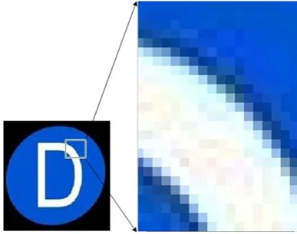
This paper focuses on zooming low resolution computed tomography (CT) scan digital images. The captured images are usually processed by digital image processors which render an image in a two-dimensional grid of pixels; characterized by a discrete horizontal and vertical quantization resolution. This finite resolution, especially for low resolution images, often results in visual artifacts, known as “aliasing” artifacts. These are very common in low resolution images and usually these aliasing artifacts either appear as zigzag edges called jaggies or produce blurring effects. Another type of aliasing artifacts is variation of color of pixels over a small number of pixels (termed pixel region). This type of aliasing artifacts produces noisy or flickering shading. A typical example of these artifacts is shown in Fig 1. These artifacts can be reduced by increasing the resolution of an image. This can be done using image interpolation, which is generally referred as a process of estimating a set of unknown pixels from a set of known pixels in an image. Image interpolation is in use for last many years, with the key interpolation techniques include linear, nearest neighbour & B-spline interpolation techniques. The typical applications of interpolation techniques include image resolution enhancement [1,2], image demosaicing [3-5] and unwrapping

Omni-images [4]. The quality of processed (zooming in this paper) images produced by interpolation algorithms depends upon the kinds of distortion and levels of degradation imposed on the interpolated image as well as the prior knowledge of the original image. The most commonly used interpolation techniques is the cubic B-spline interpolation. Analytically, it involves a cubic function, with the solution of the same depends upon the values of the co-efficient of the terms involved. This paper, therefore, is divided into two parts. The first part presents the analytical model of various interpolation functions. The second part investigates the effect of coefficients of these functions on the quality (PSNR) of the zoomed images using these functions.

Fig 1: Typical example showing the effects of aliasing on the sharp corners, when zooming operation is performed.

2.

INTRODUCING INTERPOLATION

51

Table 1. Description of various interpolation functions

INTERPOLATING FUNCTIONS DESCRIPTION

Ideal

ℎ𝑠𝑖𝑛𝑐 𝑥 =

sin(𝜋𝑥)

𝜋𝑥 = 𝑠𝑖𝑛𝑐(𝑥)

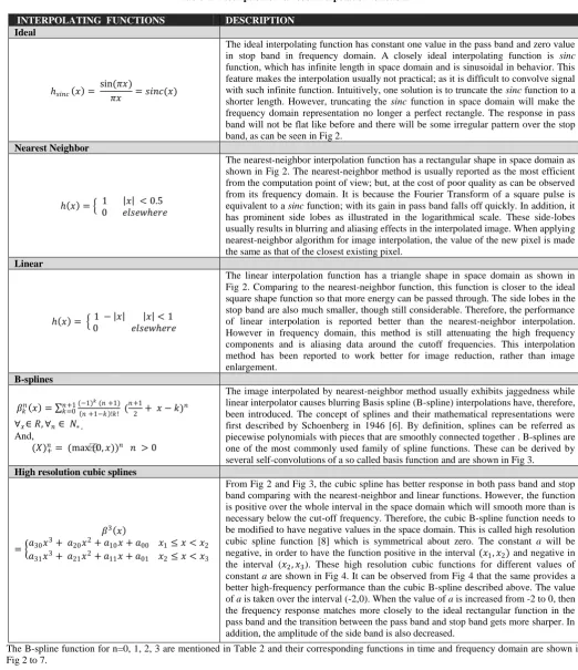
The ideal interpolating function has constant one value in the pass band and zero value in stop band in frequency domain. A closely ideal interpolating function is sinc function, which has infinite length in space domain and is sinusoidal in behavior. This feature makes the interpolation usually not practical; as it is difficult to convolve signal with such infinite function. Intuitively, one solution is to truncate the sinc function to a shorter length. However, truncating the sinc function in space domain will make the frequency domain representation no longer a perfect rectangle. The response in pass band will not be flat like before and there will be some irregular pattern over the stop band, as can be seen in Fig 2.

Nearest Neighbor

ℎ 𝑥 = 1 𝑥 < 0.5 0 𝑒𝑙𝑠𝑒𝑤ℎ𝑒𝑟𝑒

The nearest-neighbor interpolation function has a rectangular shape in space domain as shown in Fig 2. The nearest-neighbor method is usually reported as the most efficient from the computation point of view; but, at the cost of poor quality as can be observed from its frequency domain. It is because the Fourier Transform of a square pulse is equivalent to a sinc function; with its gain in pass band falls off quickly. In addition, it has prominent side lobes as illustrated in the logarithmical scale. These side-lobes usually results in blurring and aliasing effects in the interpolated image. When applying nearest-neighbor algorithm for image interpolation, the value of the new pixel is made the same as that of the closest existing pixel.

Linear

ℎ 𝑥 = 1 − 𝑥 𝑥 < 1 0 𝑒𝑙𝑠𝑒𝑤ℎ𝑒𝑟𝑒

The linear interpolation function has a triangle shape in space domain as shown in Fig 2. Comparing to the nearest-neighbor function, this function is closer to the ideal square shape function so that more energy can be passed through. The side lobes in the stop band are also much smaller, though still considerable. Therefore, the performance of linear interpolation is reported better than the nearest-neighbor interpolation. However in frequency domain, this method is still attenuating the high frequency components and is aliasing data around the cutoff frequencies. This interpolation method has been reported to work better for image reduction, rather than image enlargement.

B-splines

𝛽𝑘𝑛 𝑥 = (−1)

𝑘 _{(𝑛 +1)}

𝑛 +1−𝑘 !𝑘! ( 𝑛+1

2 + 𝑥 − 𝑘)𝑛 𝑛+1

𝑘=0

∀𝑥∈ 𝑅, ∀𝑛 ∈ 𝑁∗ ,

And,

(𝑋)+𝑛= (max⁡(0, 𝑥))𝑛 𝑛 > 0

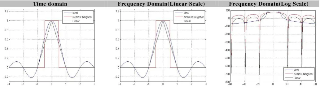
The image interpolated by nearest-neighbor method usually exhibits jaggedness while linear interpolator causes blurring Basis spline (B-spline) interpolations have, therefore, been introduced. The concept of splines and their mathematical representations were first described by Schoenberg in 1946 [6]. By definition, splines can be referred as piecewise polynomials with pieces that are smoothly connected together . B-splines are one of the most commonly used family of spline functions. These can be derived by several self-convolutions of a so called basis function and are shown in Fig 3.

High resolution cubic splines

𝛽3 _𝑥

= 𝑎30𝑥3+ 𝑎20𝑥2+ 𝑎10𝑥 + 𝑎00 𝑥1≤ 𝑥 < 𝑥2

𝑎31𝑥3+ 𝑎21𝑥2+ 𝑎11𝑥 + 𝑎01 𝑥2≤ 𝑥 < 𝑥3

From Fig 2 and Fig 3, the cubic spline has better response in both pass band and stop band comparing with the nearest-neighbor and linear functions. However, the function is positive over the whole interval in the space domain which will smooth more than is necessary below the cut-off frequency. Therefore, the cubic B-spline function needs to be modified to have negative values in the space domain. This is called high resolution cubic spline function [8] which is symmetrical about zero. The constant a will be negative, in order to have the function positive in the interval (𝑥1, 𝑥2) and negative in the interval (𝑥2, 𝑥3). These high resolution cubic functions for different values of constant a are shown in Fig 4. It can be observed from Fig 4 that the same provides a better high-frequency performance than the cubic B-spline described above. The value of a is taken over the interval (-2,0). When the value of a is increased from -2 to 0, then the frequency response matches more closely to the ideal rectangular function in the pass band and the transition between the pass band and stop band gets more sharper. In addition, the amplitude of the side band is also decreased.

52

Table 2. B-Spline Functions

n=0 n=1

𝛽0 _{𝑥 =} 1 𝑥 < 0.5 _{0.5 𝑥 = 0.5}

0 𝑥 > 0.5

𝛽1 _{𝑥 = 1 − 𝑥 0 ≤ 𝑥 < 1}

0 𝑒𝑙𝑠𝑒𝑤ℎ𝑒𝑟𝑒

n=2 n=3

𝛽2 _{𝑥 =}

−2 𝑥 2_{+ 1 𝑥 ≤ 0.5}

𝑥 2₋5

2 𝑥 + 3

2 0.5 < 𝑥 ≤ 1.5 0 𝑒𝑙𝑠𝑒𝑤ℎ𝑒𝑟𝑒

𝛽3 _{𝑥 =}

2 3−

1

2 𝑥 2 2 − 𝑥 0 ≤ 𝑥 < 1 1

6 2 − 𝑥 3 1 ≤ 𝑥 < 2 0 2 ≤ 𝑥

3.

Two dimensional interpolation for processing

images

For image processing, the one-dimensional interpolation function mentioned in Table 1 need to be transformed into two–dimensional function. The general approach is to define a separable interpolation function as the product of two one-dimensional functions [15]. To transform into multidimensional interpolation (say in two dimensions), firstly one variable is considered as fixed and then interpolation is performed along its axis (say y-axis, corresponding to y variable). This variable is then considered as fixed and then interpolation is calculated for other variable and axis, as shown in Fig 5. Finally, all the obtained functions are then combined to have:

) , ( ) , ( ) , ( ) , ( ) , ( 2 2 1 2 1 1 2 1 2 1 1 2 1 2 1 2 1 2 2 1 2 1 2 1 1 1 2 1 2 2 1 2 y x f y y y y x x x xi y x f y y y y x x x x y x f y y y y x x x x y x f y y y y x x x x y x f i i i i i i i i i                     (1) } ) ( ] 4 ) 1 )[( ( ] 6 ) 1 ( 4 ) 2 )[( ( ] 4 ) 1 ( 6 ) 2 ( 4 ) 3 )[( ( { 6 1 ) , ( 3 ' 2 1 3 3 ' 1 1 3 3 3 ' 1 3 3 3 3 ' 1 1 y x f y y x f y y y x f y y y y x f T y x f                    (2)

Where, 0 ≤ 𝑥 ≤ 1; 0 ≤ 𝑦 ≤ 1, T = sampling duration,

𝑓 𝑗 𝑥 =_6𝑇1 𝑏3𝐼 𝑖𝑗∗ 𝑥3−𝑖, 𝑗 = 𝑙 − 1, 𝑙 + 1, 𝑙 + 2, (3)

And

𝑏𝑗 = 𝑈 ∗ 𝑐𝑗; and 𝑈 =

−1 3 −3 1

3 −6 3 0 −3

1 4 0 3 01 0

(4)

Where

𝑏𝑗 = [𝑏0𝑗, 𝑏1𝑗, 𝑏2𝑗, 𝑏3𝑗]𝑇 and 𝑐𝑗 = [𝑐𝑘−1,𝑗, 𝑐𝑘,𝑗, 𝑐𝑘+1,𝑗, 𝑐𝑘+2,𝑗]𝑇

This 2D interpolation function is termed as bilinear Lagrange form equations[12-14]. Using this method, the cubic interpolation (Table I) in two dimensions [9-11] can be written as per Eq. 2, 3 & 4.

The values of b & c matrix [15-16] can be computed by substituting x=0 and y=0 in equation (2) above. The time and frequency domain (linear & logarithmic scale) representation of linear, nearest neighbor, bilinear, Cubic B-spline (n=0,1,2,3) interpolation function and high resolution cubic B-spline functions (a=-2, -1.5, -1, -0.5 & 0) in two dimensions are shown in Fig 6 and Fig 7. These functions are then applied to CT scan image. The results obtained are shown in Fig 8 and Fig 9. A discussion on the results obtained is presented in next section.

Time domain Frequency Domain(Linear Scale) Frequency Domain(Log Scale)

53

Time domain Frequency Domain

(Linear Scale)

Frequency Domain (Logarithmic Scale)

Fig 3: The time and frequency domain cubic B-spline interpolation techniques for n=0, 1, 2 and 3.

Time domain Frequency Domain

(Linear Scale)

Frequency Domain (Logarithmic Scale)

Fig 4: The response of high resolution cubic B-spline interpolation function for a between -2 & 0.

54

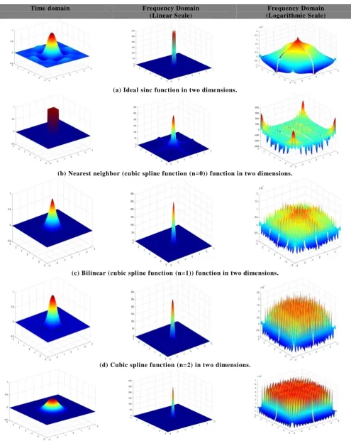
Time domain Frequency Domain

(Linear Scale)

Frequency Domain (Logarithmic Scale)

(a) Ideal sinc function in two dimensions.

(b) Nearest neighbor (cubic spline function (n=0)) function in two dimensions.

(c) Bilinear (cubic spline function (n=1)) function in two dimensions.

(d) Cubic spline function (n=2) in two dimensions.

(e) Cubic spline function (n=3) in two dimensions.

Fig 6: The time domain and frequency domain (linear & logarithmic scale) response of (a) Ideal, (b) Nearest neighbor and Cubic spline function for n=0, (c) Bilinear and Cubic spline function for n=1, (d) Cubic spline function for n=2 , and (e)

55

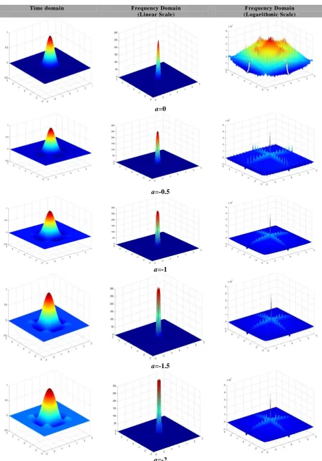
Time domain Frequency Domain

(Linear Scale)

Frequency Domain (Logarithmic Scale)

a=0

a=-0.5

a=-1

a=-1.5

a=-2

56

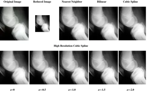
Original Image Reduced Image Nearest Neighbor Bilinear Cubic Spline

High Resolution Cubic Spline

a=0 a=-0.5 a=-1.0 a=-1.5 a=-2.0

Fig 8: A CT scan image of knee is reduced to 50% of its original size and then zoomed back to its original size using nearest neighbor, linear, cubic and high resolution cubic spline with a=0, -0.5, -1, -1.5 and -2.

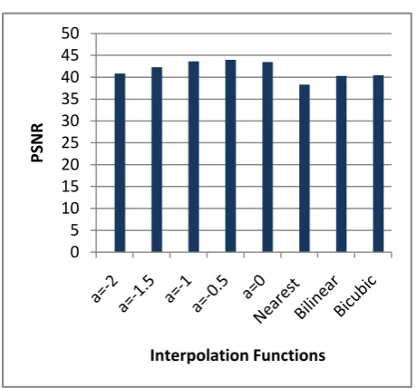
Table 3. PSNR of images zoomed using Nearest Neighbor, Bilinear, Bicubic and High resolution cubic spline 2 dimensional interpolation function

a=-2 a=-1.5 a=-1 a=-0.5 a=0

40.8679 42.3022 43.638 43.9643 43.471 Nearest Neighbor Bilinear Bicubic

38.3138 40.2942 40.4279

4.

RESULTS AND DISCUSSIONS

In order to investigate the characteristics of the nearest neighbor, bilinear, cubic spline and high resolution cubic spline functions with a between -2 to 0 (inclusive), the same are implemented in Matlab. Their response in time domain and frequency domain in one dimensions and two dimensions are computed and shown in Fig 2 to 7. In frequency domain, the response of these functions is evaluated on both linear and logarithmic scale. The linear scale is used to show the pass band performance; whereas, the logarithmic scale shows the stop band performance. From Fig 2 to 7, it is found that with respect to ideal interpolation function, the high resolution cubic spline functions have shown the best response in the pass band. It is observed that for the parameter a=-0.5, the response is flat at the intermediate frequencies. However, when the value of a is further decreased to -2, then the cut off frequency is traded for a more rapid transition between the pass band and stop band. In comparison to ideal and linear functions, the nearest neighbor function has a better response in the pass band; however, it offers more attenuation even at very low frequencies. Both the bilinear and cubic B-spline

Fig 9: PSNR comparison of image of Knee zoomed using nearest neighbor, bilinear, cubic and high resolution cubic spline 2 dimensional functions.

5.

CONCLUSION

From the analytical functions and their graphical representations in time and frequency domain (linear and logarithmic scale), the nearest neighbor function does moderately well in the pass band; however, has comparatively higher side lobes in the stop band. The bilinear interpolation function performs comparatively better in the stop band; however, at the expense of considerable amount of smoothing in the pass band. The cubic B-spline has better stop band performance than nearest neighbor and linear; however, it has wider pass band. The high resolution cubic splines have the best combination of both pass band and stop band performance. However, this is observed for a=-0.5. In situations, when a is further decreased towards -2, then the function has a significant degradation in its response in both pass band and stop band. These functions are applied on a CT scan low resolution image with a zooming factor of 2. It is observed that the visual results of high-resolution cubic spline interpolation with a=-0.5 are better as compared to nearest neighbor, bilinear and cubic spline functions. The PSNR corresponding to this function is also more than others as shown in Fig 9. However, it is computationally expensive. In addition, it is also observed that the nearest neighbor algorithm has the shortest extent in the image domain, one interpixel distance. The linear interpolating algorithm, extends over two interpixel distances; whereas, the high resolution cubic splines extends over four interpixel distances. In concern to zooming operation, the performance of the discussed interpolation functions can be arranged in a sequence as high resolution>cubic spline>bilinear>nearest neighbor.

6.

REFERENCES

[1] M. Hanumantharaju, M. Ravishankar, D. R. Rameshbabu & S. Ramachandran, “Color Image Enhancement using Multiscale Retinex with Modified Color Restoration Technique,” Second International Conference on Emerging Applications of Information Technology (ICEAIT), pp. 93-97, 2011.

[2] Z. Min, W. Jiechao, L. Zhiwei & L. Yonghua, “An Adaptive Image Zooming Method with Edge Enhancement,” 3rd International Conference on Advanced Computer Theory and Engineering (ICACTE), pp. 608-611, 2010.

[3] Wing-Shan Tam, C. W. Kok & W. C. Siu, “A Modified Edge Directed Interpolation For Images,” 17th European Signal Processing Conference (ESPC), 2009.

[4] W. Bender & C. Rosenberg, “Image Enhancement Using Non-uniform Sampling,” Proc. SPIE-int. Soc. Opt. Eng., Volume 1460, pp. 59-70, 1991.

[5] P. Thvenaz, T. Blu & M. Unser, “Image Interpolation and Resampling,” Handbook of Medical Imaging, Processing and Analysis, I.N. Bankman (eds.), Academic Press, San Diego CA, USA, pp. 393-420, 2000.

[6]

[7]

M. Zamani, “An Applied Two-Dimensional B-spline Model for Interpolation of Data,” International Journal of Advanced Research in Engineering and Technology (IJARET), Volume 3(2), July-December 2012.

R. G. Keys, “Cubic convolution interpolation for digital image processing,” IEEE Trans. Acoust., Speech, Sig. Proc., Volume 29(6), pp.1153-1160, 1981.

[8] R. W. S chafer & L. R. Rabiner, “ A digital sign al processin g approach to interpolation,” Proc. IEEE, Volume 61, pp. 692–702, 1973.

[9] T. Acharya & P. S. Tsai, “Computational Foundations of Image Interpolation Algorithms,” ACM Ubiquity Volume 8, 2007. [10] T. M. Lehmann, C. Gonner & K. Spitzer,

“Interpolation Methods in Medical Image Processing,” IEEE Transactions on Medical Imaging, Volume 18(11), pp. 1049-1075, 1999. [11] J. Anthony Parker, R. V. Kenyon & D. E. Troxel, “Comparison of Interpolating Methods for Image Resampling," IEEE Transactions on Medical Imaging, Volume 2(1), pp. 31-39, 1983.

[12] E. Maeland, “On the comparison of the interpolation methods,” IEEE Trans. Med. Imag., Volume 7(3), pp. 213-217, 1988. [13] M. F. Fahmy, T. K. Abdel Hameed & G. F.

Fahmy, “A Fast B-spline Based Algorithm for Image zooming and Compression,” 24th National Radio Science Conference (NRSC), Egypt, 2007.

[14] H. S. Hou & H. C. Andrews, “Cubic Splines for Image Interpolation and Digital Filtering,” IEEE Trans. Acoust., Speech, Signal Processing, Volume 26, pp. 508-517, 1978. [15] S. E. Reichenbach & S. K. Park,

“Two-parameter cubic convolution for image reconstruction”, Proc. SPIE, Volume 1199, pp.833-840, 1989.

[16] M. Unser, “A Perfect Fit for Signal/Image Processing: Splines," Proceedings of the SPIE International Symposium on Medical Imaging: Image Processing (MI'02), 4684, Part I, pp. 225-236, San Diego CA, 2002.

0 5 10 15 20 25 30 35 40 45 50

PS

N

R

Interpolation Functions