Software Project Contacts by GRGA Scheduling and EVM

Software Project Contracts and Scheduling by GRGA

and EVM

Dinesh Bhagwan Hanchate

Baramati, Pune

Rajankumar S. Bichkar

Pune, India.

ABSTRACT

The well planned SPLC (Software project life cycle) doesn’t give certainty about the completion of project in time and budget. The PMP (Project Management Processes), pregnant processes, rework, some float types and review process, always, put stum-bling block for completion of project in Time. Apart from this defined process, there is need of genius decision making pro-cess. The various planned schedule, redundancy and contingency target schedules can be used as input for decision making pro-cesses and the solutions to be adapted during the stages of SPLC. This paper gives various schedule types with respect to software project contracts. These schedule types are the outputs of GRGA (Gene Repair Genetic algorithm) along the utilisation of EVM (Earned Value Management) concepts. The GRGA (Gene Repair based Genetic Algorithm) approach gives choice to change the constraints and or features as objective components in objective function. In this paper, we present different schedules as the out-come to evaluate the effectiveness of genetic operator GeneRe-pair. This operator is developed to correct invalid schedule gen-erated following crossover and mutation. Following implemen-tation and testing of GA with GeneRepair, we found a signif-icant positive side in our results in speed and accuracy also. we have been able to generate very good results in an efficient manner, in terms of both time and number of evaluations us-ing GeneRepair with traditional crossover and mutation operators.

General Terms:

Software Project Management, Machine learning

Keywords:

PMP, Software Contacts, GRGA, COCOMO, SPSP (Software Project Scheduling problem), Constraints Optimization, EVM.

1. INTRODUCTION

Cognizant engineers and software managers are often in the business of scheduling a series of engineering task. In constructing good schedules, management requires satisfactory schedule plan. The standards algorithms are too consuming for any practical use for getting an optimal schedule. A machine learning technique called genetic algorithm is iterative, Meta-heuristic search method

which gives the near optimal solution to a problem. GRGA [24] approach is considered, in this study, to get and generate various schedules for software engineering project for various combination of features considered under the different circumstances of ACWP (Actual Cost of Work Performed [1]). These schedule plans or types are related with time constraint, cost constraint, with time-cost-skill constraint, time- cost skill-overloading constraint and others plans. This paper imparts various near optimal schedules which give alternative schedule choice to PM to adapt any solution according to the situation and constraints required by project scope and concerned contract.

This paper addresses some issues, these are

?Study of Software contracts, PMP, scheduling plan & estima-tion [2] [47].

?EVA used in proposed approach based on EVM by Anita [45], Hughes [11] and SEE principles by Bohem principle

?Importance of Gene repair.

?pros and cons of GRGA and COCOMO-II solutions.

?The work is studied and derived from that of[ Carl 2001] [9], we do take opportunity to do the experiments for comparison and similarities with proposed approach by adding some features.

The paper is arranged as follows

•section I gives introduction part.

•section II gives the theory and Hypothesis for proposed GRGA approach and PMP [1].

• section III discusses about GA, Gene Repair and proposed GRGA.

•section IV puts light on assumptions and problem definition for Proposed approach.

•section V gives study of various schedule types.

•section VI describes results and discussion.

•section VII gives future direction along with conclusion.

•section VIII is about concerned reading, work, inspiration and support by Machine learning related authors.

2. THE THEORY AND HYPOTHESIS 2.1 Project Management Processes [4]

Table 1. Notations, symbols and meanings [45] [18] [17]. Notations Meaning

WBS Work Breakdown Structure MM man-months

FSP Full Time software professional KDSI Thousands of delivered

source instructions TDEV Development time HCTi Head Count

SPLC Software Project Life Cycle CDTi COCOMO Calculated duration

of task Ti

GRODTi Optimistic duration of task Ti obtained by GRGA approach CPDTi COCOMO pessimistic duration

of task Tiand equal to 1.6×CD DUR Project duration

EDURavg Expected project DUR

.

=CEDTi

TPHC Total project head count. EMF Effort multiplier factors sth _{Schedule number in generation} Pc Crossover rate

Pm Mutation rate FCs Fitness of sthSchedule Ps Total Penalty of sthschedule SP Size of Population

SalEEj Maximum salary of employee among all employees TTs Total time of sthschedule OTs Over time of sthschedule

considered as penalty TCs Number of Task completion of

sthschedule

GRDLCs DLC of sthschedule by GRGA CDLCs DLC of sthschedule by COCOMO

µ Overtime penalty rate

η Time penalty rate TPs, Time Penalty

of sthschedule

TCHCs Total COCOMO head count of sth_schedule

GRSHDs Schedule obtained by GRGA approach of sthschedule

CPSHDs COCOMO pessimistic of sthschedule COSHDs COCOMO optimistic of sthschedule SPI Schedule Performance Index SV Schedule Variance CB Cost Baseline CPI Cost performance Index BAC Budget at completion

CEVP Cost Estimate Validation Process

ICC (Integrated Change Control) activities. Ultimately at the end,the SM (Software Manager) /PM will check the total and entire completed work. He confirms the objectives are met or not; this can be achieved by the various studies of schedule types which is produced here by EVM (Earned Value Management [11] [6]). According to PMBOK, there are five Project Management Pro-cesses [1], are must for any type of project. These five Project

Table 2. Notations,symbols and meanings [45] [18] [17]. Notations Meaning

CMP Cost Management Plan AC Actual Cost

EV Earned value or approved or budgeted cost CPF Cost-plus-fee

CPFP Cost-plus-fixed fee CPIF Cost-plus-incentive-fee PEV Proposed Earned value CEV COCOMO Earned Value GREV EV obtained by GRGA Approach AC Actual Cost

PDM Precedence Diagramming Method SCE Software Cost Estimation PEV Proposed EV

CEV COCOMO-EV

CTT COCOMO Threshold Time ET Estimated Time

SM Schedule Margine CM Cost Margine

SHD the post fix word SHD in some notations give array of tasks assignment to employees. GRDs Total time of sthGRGA schedule

Total Time Total time (in figs. and tables) is GRD except simple time ST-2 type

GRCTs Critical time by GRGA

GRCT is CT obtained and shown in respective schedule sections in figures

Pr profit

C Constant

TO Turnover

Prior History of clients CDC Cost oriented contract TDC Time oriented Contract.

Management Processes are though different in nature with any Project Phases life Cycles as these processes are dependent on industry.

These processes can be embedded in every stages of SDLC [30]. These five groups become important part of the SDLC. The MPG (Monitoring Process Group) is responsible for potential performance of projects in terms of schedule and costs. Hence, the proposed approach uses this group for suitable schedule type. Any project starts with the Initiating Process Group where it is de-cided if the project will be selected and accepted based on high-level planning efforts performed at this stage. If the project is ap-proved, it will move further to the Planning Process Group, so de-tailed Project Management Plans are prepared. The Executing Pro-cess Group will follow, so the work will be completed according to the plans. The results will be supplied to the Monitoring and Con-trolling Process Group that will make sure the project is on the track in terms of scope, time, cost, risk and quality. In the case when vari-ations to the plan are encountered, depending on the severity of the identified issues, the project will return back to Initiating , Planning or Executing. Following part of the section explains briefly the all processing groups.

users requirements and their needs, objectives, high level costumor needs, summary BAC, milestones, risks and so on, so forth. All these items are the parts of the project charter. The change in above items in turn affects on several components. But, these components can be managed as distinct and uniform projects since it has sepa-rate requirements, budgets and cost. Even though the collecting the requirements usually is part of planning phase, the requirements elaboration, specification and clarification stage start actually, here, in order to make available for the charter. The nonfunctional and functional requirements, packages, tools and delivery dates are de-cided in this group.

2.1.2 PPG (Planning Process Group). Once the approval is given to the charter document, the development will propagate from IPG to the Planning step. From this point, the analysis starts by identifying the domain and scope of the individual projects. This stage finalise the actions to be performed in order to satisfy and meet the requirements, so the approved PMP (project manage-ment plans) will be in hand. These PMPs include requiremanage-ments re-finement, BAC, quality requirements, risk identifications, defined scope, WBS creation, schedules, response planning etc.

The analysis part generates a unique and Integrated SRS (Software Requirement Specification) document (at the program level) which describes the use cases with actors and processes. This document is very useful as basis for generation of the test cases. Right after this, the WBS creation will start to make them detailed at feature level. The analysis part will be then continued with a detail and comple te clarification of requirements. A SRS dedicated document will be created for each delivery for designing the test cases. This docu-ments split the features by generating HLD (High Level Design) documents. so,at the end, the WBS latest will be filled in.

2.1.3 EPG (Executing Process Group). The execution activities is performed at the Project and Delivery level. The project will be-gin with the first Delivery, and followed by second Delivery. This continues with number of deliveries in the projects. Once a compo-nent is entirely implemented and seen, it will be prorogated further for the the inspection and validation. Even though an intermediate tests are conducted for QC, but these tests cannot be replacement of the full inspection of delivery package.

2.1.4 CPG (Controlling Process Group). 1.Project Level : Qual-ity Control will be performed at this level, so a strong and stringent quality check will take place for each and every delivery (each com-pletion of milestones) of a project. So, these are managed at this level. The Quality Control Department has role of assembling the individual components into a single package corresponding to the entire project delivery. This is called as integration of project. Inte-gration testing activities will generate Test Results, Test Evaluation Reports and other documents, too, if needed.

2.Program Level: A second QC (Quality Control) step will be per-formed at this level, in order to confirm the validation of pack-ages of each project are really working bilaterally and together as a whole. Some packages which dosn’t pass QC test may be rejected, so they will send back to Executing or Planning stages depending upon the results of test.

2.1.5 MPG (Monitoring Process Group) [32] [45]. In order to see the potential performance deviation of its corresponding projects in terms of schedule and costs, by starting from the fol-lowing values the EVM (Earned Value Management) method is ap-plied: EV (Earned Value), PV (Planned Value), AC (Actual Cost). The Schedule Variance (SV), Schedule Performance Index (SPI), Cost Variance (CV) and Cost Performance Index (CPI) are useful

for measuring the deviations of project deviations in terms of cost and schedule, so these indicators are useful and can be used to show how the project takes path with respect to contract with the client.

2.1.6 CLPG (Closing Process Group). Project closing assists to PMs to make assurance of all the program work is completed. It also make sure that objectives for the projects have met right from starting of the charter and project management plans. All the changes and updation must be reflected in the entire program tech-nical and non techtech-nical documentation, including the plans. The updated and historical information, record and statistics should be documented as these files for program and projects archived can be useful for future use. The acceptance of customer should be in-cluded, too, as well as the formal completion of project documenta-tion. Finally and last, the project or and process improvement ideas is collected from the stakeholders. The program teams will be in-formed and communicated about the end of the project, also, the releasing of future new assignments.

2.2 Types of Contracts [3] [51]

There is a need of establishing business deals and partnerships in this today’s world of business. This can be done by contracts. The contract types are decided by the parties involved in the business engagement. In ground reallity and matter of fact, the type of the contract used for the business engagement varies mostly depending on work type and industrial nature. The contract is nothing but it’s an logical and elaborated understanding and agreement between two or more parties. One or more parties may provide products or services in return to something provided by other parties (client). The contract type plays the key role in relationship between the parties engaged in the business and the contract type determines the project risk [22].

Let’ us see most widely used contract types in all engineering in-dustries as well in software industry.

2.2.1 Fixed Price (Lump Sum). This is one of the simplest con-tract type. The terms are quite simple, straightforward and not so difficult to understand. The SP (service provider) agrees to provide a defined service for a decided or specific time period. The client gives word to pay a fixed amount for the service. This contract type may decide certain milestones for the deliveries and also KPIs (Key Performance Indicators). In addition, the software contractor may have his(r) an acceptable criteria defined and fixed for the mile-stones and the final delivery. The main significance of contract type is that the client knows the total fixed project cost before the project starts.

2.2.2 Incentive. An uncertainty in project cost is the main cause and reason of making this type of contract. The technological chal-lenges gives effect on all effort and resources though there are ac-curate estimations in this contract. There are three cost factors in an Incentive contract; target price, target profit and the maximum cost. Both the parties should feel ease as this contract device tar-geted price overrun between both. The SP and client helping hand provides to minimise the risks in the business for both parties.

make the agreement and signs off the estimate with d Statement of Work (SOW), the service provider can have green signal to start work. The T&M contracts are nearly utilized for long-periodic and tenure business engagements. This is not possible other contracts.

2.2.4 Unit Price. In this contract, the entire project is divided into units. The each unit or milestone is defined. This contract type can be placed and introduced as one of the more flexible methods compared to fixed price contract. Usually, the contractor and client of the project decides on the cost estimates. Both the parties asks the bidders to make bond and bid of each element of the project. After making bond and bidding, depending on the bonded amounts and the qualifications of bidders. The entire project may be given to different providers or the same service provider. Different units may be assigned and allocated to different SPs. This contract is really becomes important when different project units or milestones require different specialists and expertise to complete the project.

2.2.5 Cost Plus. The services provider is reimbursed for their labour, machinery and other costs. In this model, the agreed fee has to be paid by contractor to the service provider. The detailed schedule has to be provided by the service provider. The resource allocation for the project is given by SP also. Periodically reporting to the contractor is must regarding all the costing in the budget of project. The payments may be paid by the contractor at a certain frequency (such as monthly, quarterly) or by the end of milestones.

2.2.6 Percentage of Construction Fee. This type of contracts are especially utilised used for engineering projects. Based on the re-sources and material required, the cost for the construction is esti-mated. Then, the client pays a percentage of the cost of the project as the fee for the service provider after the agreement. As an ex-ample, take the scenario of construction of home. Assume, the es-timate comes up to Rs.4,00,000/-. When this project is contracted to a service provider, the client may agree to pay 25 PC of the total cost as the construction fee which comes up to Rs. 1,00,000/-.

2.3 The Schedule management

Though, our approach is considering the direct cost, we emphasise on the adjustment of cost budgeting which is the combination of both direct and indirect costs. Ultimately, the cost of the complete project is combinations of the factors related to these both costs. We want to give free hand to PM for getting correct contingency plan for cost and time for different schedule plans with different contracts. ACWP is originally considered as direct cost which is related to labour cost only. But, some companies may take the AC as the combination of the both the direct and indirect costs. We re-fer the latter one AC for proposed approach so that we can have different schedule types in the hand of PM depending upon how the PM decides to cut the angles of features (including time and cost). The Schedule management in SPM (Software project Man-agement [50]) consists of criteria and the activities, used for devel-opment of software project, are based on the needs of the project. The schedule management consists of schedule activities, its analy-sis, technique (making time span short), schedule control (process). Not only, these factors but also, SPI (Schedule Performance Index), SV (Schedule Variance) give idea how to control the project with various schedule by mean of DUR (duration of project).

SP I=EV

P V (1)

SV =EV −P V (2)

Table 3. INPUT:Task Properties [9]. Task Efforts CD CPD Required

id (PM) Months Months skills

0 10 6 9.6 1,2

1 15 7 11.2 3,4

2 20 8 12.8 4

3 10 6 9.6 1,3

4 15 7 11.2 2,3,4

5 15 7 11.2 1,3

6 10 6 9.6 2,4

7 10 6 9.6 1,5

8 20 8 12.8 3,4

9 20 8 12.8 3,5

10 10 6 9.6 1,2

11 15 7 11.2 3,5

12 20 8 12.8 4,5

13 25 8.5 13.6 2,5

14 15 7 11.2 4,5

15 10 6 9.6 2,4

16 15 7 11.2 2,5

17 10 6 9.6 2,3

Table 4. INPUT:Employee property table [9]. Employee Salary Month Overload skills

id

1 5000 1 1.1 3,4

2 4000 1 1.15 1,3

3 3000 1 1.2 2

4 5000 1 1.15 3,4,5

5 3000 1 1.15 1

6 6000 1 1.15 2,3,4

7 6000 1 1.15 2,3

8 5000 1 1.15 2,3,4

9 8000 1 1.15 2,3

10 9000 1 1.15 1,2,5

where, EV is earned value and PV is planned value. The SPI or SV are used to see the performance of the project schedule. If SPI>1 and SV>0 then it indicates, project is within controlled plan in real development SPLC time [32]. This is dependent upon baseline, the approved plan for project, WBS (work breakdown structure), it’s components and target schedules. SPI and SV can used for calcu-lation of fitness for getting target schedule, also [35].

2.4 Baseline

The baseline includes cost, DUR and scope of the project. Vari-ous schedules are inputs to the baseline of software projects. The types of schedule can be used and adapted in the baseline depend-ing upon the scope baseline, scope change, scope control, scope creep. All above scope management activities give opportunity to PM (project manager) to adopt the schedule type accordingly. Con-tingency allowances give also space to PM to adjust in fullback position by using the money or time and both for coming up from the overrun. Contingency plan gives 10PC on DUR or cost as the contingency plan dependent on CB (cost baseline).

2.5 Software Cost and budgeting

impor-tant part of RE (Requirement Engineering). This uncertainty relates with cost growth and negative CPI (cost performance index [35]), are main reasons of inaccuracy in the cost estimation and schedule cost. The software requirement engineering is the important part for getting the requirement analysis in clear manner so that, we can improve budgeting by requirement specificity for keeping the ac-curacy in estimating, efficiency of costing i.e. with keeping CPI in better range. Another uncertainty, in the software cost estimation is making under-estimation of software size (KLOC). The study of Hihn and Habib shows that best estimation is mean estimation of underlying effort. BAC (Budget at Completion) is sum of the es-timated cost of every tasks or work to setup cost baseline as cost baseline is the part of main baseline. CEVP (cost estimate valida-tion process) is another way of making the cost/budget fixing and is the part of CMP (Cost Management Plan), in turn; CMP is the part of project management plan. This plan and process can be ad-justed with each CPI of every phases during the project develop-ment in SDLC. Just like SPI [32], CPI gives measuredevelop-ment for cost efficiency and is defined as

CP I=EV

AC (3)

where EV and AC are in target scheduling. AC is expenditure cost also. Keeping various EV value , we can have different schedules. PM can see the contingency plan where schedule cost and DUR will affect on CPI as actual cost includes various contract fea-tures and method. These contracts are CPF (cost-plus-fee) contract, CPFF (cost-plus-fixed-fee ) contract, CPIF( Cost-plus-Incentive-fee) contract. These reimbursable contracts are always the part of the cost budgeting. These types of contracts gives PM to move around in the schedule plan for making the trade-off between vari-ous schedule planes and schedule cost in baseline (original or first or basic plan) at construction (build) phase of SPLC. As SPI can be used for the fitness in target scheduling, CPI can be used in adjust-ing the indirect cost.

2.6 About SCE and it’s step [31] [43] [49] [7]

Software cost estimation plays different role at different stages or phases of SPLC. Schedule plan or even baseline of SCE is depen-dent on different role at different stages or phases of SPLC . In early stage of SPLC, generally emphasize is given on design related part and later on it becomes the part of management i.e. scheduling.

·Schedule Cost Estimations may be done by an expert or team of specialists, analytical way of historical data, various models along with thumb rules.

·Some industries satisfies with PC effort estimation by phase wise. There is standard PC distribution of effort, can be taken from Uni-form Software project management phase wise distribution table.

·This phase wise or WBS wise estimation may be done by tak-ing parametric cost models or by mathematical relationships. This type of estimation has relations of parameters at various levels and stages of projects of similar or same type. These typical parameters are defined for specific type of projects. The relation between them gives mathematical model expressions for every phases.

·Historical analogy estimation methods are dependent on effort, phase wise cost of past projects which are completed successfully.

·Expert judgment is another way of doing estimation as the experts are related to their domain.

♣Steps of Software cost estimation [6]

Software estimation consists of many tasks and functions to do in systematic steps. Elicitation of information, requirements, defining the work elements, software size estimation, estimation of effort,

scheduling of effort, cost estimation, determination of risk effects, validation of estimation or budget by analogy, reconstructing the budget and schedule, reviewing and approval of estimates, moni-toring the cost expenditure Vs budget allocated maintain the lin-earity in it [7] [30]. These are all the steps in software estimation which are the part of software schedule plan it self. Among these, we are concentrating on scheduling plan which is the prime work of software manager, estimator, cognizant engineer.

2.6.1 Scheduling the Effort. This is the main part of the project cost estimation where we have to calculate the time required to complete the project according to WBS. Every WBS has work el-ement with proposed time requirel-ement. Letting of 10 PC of sched-ule time is generally allowed as margin as it is regular practice. One month is given margin for one year schedule. Determining the order or sequence is the next step. The dependencies between activities and WBS components are also in the drive. The project schedule margin is considered to adjust the CT (Critical Time) and pessimistic duration in which, the CT is calculated by PDM (prece-dence diagramming method). CT is longest path in the activity net-work of schedule and can be taken as threshold for the completion of the project.

2.6.2 Calculating the Direct Cost (ACWP). This step has some sub steps. These are determination of cost procurements, cost pro-posed training period, determination of salary and skills profi-ciency. It is necessary to iterate the estimation several times by iter-ative methods. This estimation is cost value EV. 55 PC of projects goes beyond the budget (EV) that to by over and above 90 PC (ac-cording to Remer [3]). 8 to 18 PC time should be given to develop-ing the plan also, dependdevelop-ing on technology used for project.

2.6.3 Validating the Estimate. The thumb rule tells to keep al-ternate estimation technique for comparison, these may be and are expert opinion estimation and model-based estimations. We can do comparison of our estimated cost with any other model. Generally, comparison parameters are size, effort, and cost of same type of projects. Resolving the differences, reviewing-refining the sched-ule and schedsched-ule plan are continuous process in SPLC and to be done as regular checkpoint. That’s why we developed plans for not only for baseline also for target scheduling. Proposed model can be , also, used as target scheduling model.

2.6.4 Reconcile Estimates, Budget and Schedule. Cost of indi-vidual functions, precedence of it, inter communications are con-sidered in this step. In real practice, one should reduce the func-tionality to reduce the function points in terns to get the tasks to accommodate in budget. Budget margin calculation is done as fol-lows

CostM argin=(P EV −CEV)

P EV . (4)

ScheduleM argin=CSHD−GRSHD

CSHD (5)

where PEV= proposed EV, CEV= COCOMO-EV,

CTT=COCOMO Threshold time, ET=estimated time. Above margin is used for minimizing the cost and time for calculating the fitness of individual schedule plan

3. GA, GENEREPAIR AND GRGA [28] [25]

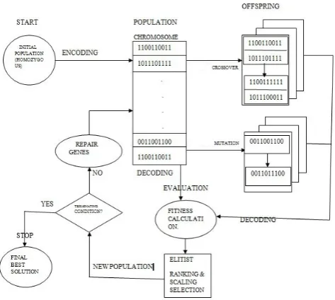
Fig. 1. Proposed GRGA Approach

GA can be shown as fig.3. The evaluation function does a heuristic estimation quality solution. The search process is completely taken in the hand by the variation and the selection operator.

3.1 GA Components

GA consists of representation i.e. representation and definition of individuals , evaluation function means fitness function or com-pound function, population, next generation individuals i.e. parent selection mechanism, variation operators (crossover and mutation), survivor selection mechanism (replacement) [37] [24].

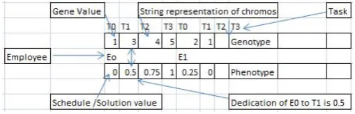
3.1.1 Representation. Phenotypes are types forming possible so-lution within space of original problem. The encoded individuals in the GA evaluation are called genotypes. The representation is the mapping from set of the phenotypes onto a set of genotypes. Possi-ble solutions consists of Candidate solution, phenotype and individ-ual. This entire space is knows as phenotype space. Chromosome, and individual are the points in the genotype space. Single unit el-ement in a chromosome is called gene. A gene value is called an allele. This representation is shown in fig.4.

3.1.2 Variation Operators. The role of variation operators ( crossover and mutation) is to create new generated individuals from past and old ones.

1. Mutation Operator : Mutation is a unary variation operator to apply on genotype. It produces the child or Offspring. Mutation is important operation which can guarantee about connected space. 2. Crossover Operator : Crossover or some time called recombina-tion is a binary variarecombina-tion operator which merges informarecombina-tion from two parent genotypes which leads and results into one or two off-spring genotypes. Similarly to mutation, crossover is also stochastic operator. The random drawings are significance in this operation as choosing the parts of each parent, combining them and it’s way and method depend on random drawings. The purpose of crossover is of mating two individuals which are different but having desirable fea-tures . This operation produces an offspring which combines both the features.

3.1.3 Parent Selection Mechanism. The role of parent or mat-ing selection is to make comparison and distmat-inguish among indi-viduals based on their quality which allows the better indiindi-viduals to become parents for forthcoming generation. The mating selec-tion is based on probability and high quality individuals get a more chance than those of lower quality to become parents. Nevertheless, selection gives small but positive chance to low quality individuals, otherwise the complete search can get block and stuck in a local optimum.

3.1.4 Survivor Selection Mechanism. As opposed to stochastic parent selection, survivor selection is always deterministic. e.g., ranking the unified multiset of parents and offspring which selects the quality and top segment (fitness biased).

3.1.5 Initialization. Initialization is generally put in simple form in most GA applications. This steps requirement depends on appli-cation at hand as it may be result in extra computational effort or not so much also.

3.1.6 Population. As population is a genotype multiset, the func-tion of the populafunc-tion is to keep possible solufunc-tions. Usually in all GAs applications, the size of population is kept constant.

3.1.7 Termination Condition. As GA is stochastic and mostly, there are seldom guarantees to get an optimum way and solution. The following are the commonly used terminations conditions and These are as :

1. if the maximum letting CPU times elapses. 2. if The fitness evaluations reaches a given limit.

3. if the fitness improvement get stuck up at same value and keep itself under a threshold value,for a given period of time.

4. the population diversity goes down and drops under a given limit and threshold.

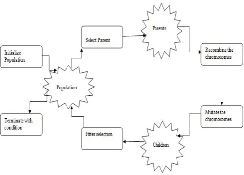
The traditional and simple GA is given as below in algorithm and also diagrammatical representation in fig.3.

Fig. 2. Genetic Algorithm.

4. ASSUMPTIONS, BUILDING BLOCKS AND PROBLEM DEFINITION FOR PROPOSED GRGA APPROACH

The GRGA operates in traditional genetic algorithms manner, and is simply summarized as follows and shown in fig.1:

Fig. 3. Diagrammatical presentation of Simple GA.

individuals in the population lies solely with the GeneRepair operator.

As, proposed GRGA approach [24] gives the direction to cognizant engineers and estimators for differentiation and deviation between two estimation models. Thats why, we proposed different types of schedule with various constraints and conditions which gives alternative ways to show to the top management in different scenarios. Schedule types are based on single variable constraints, multiple variable constraints, non-constraint objective function type optimization techniques involved in genetic algorithm. Single variable constraint or single objective component function can be solved by other optimization techniques also. These techniques are linear programming, convex or concave optimization technique for two variable optimization. There are some cases or situations where we dont want to optimize anything. This type of feasibility problems only satisfies constraints to the model and not having objective. So the schedules are only dependent on soft and hard constraints . The example is problem solved for skill matching taken as hard constraint. Another type of objective function is multiple objective functions, are used to optimize number of different objectives simultaneously [39].

For optimization problem, variables are essential than the con-straints [40]. We considered also functional concon-straints and side constraints also. As, the functional constraints are behavioural constraints which gives boundaries to the performance of a system rather than using the behavioural constraints, we used side constraints which is applicable for schedule design variables e.g. availability of a skilled staff.

Suppose∃A, B,C the sets of real or integer valued data for respec-tive and particular range of the variables. As we have taken set T = number of task,E = number of employees, Sk= set of skills. All these sets are to be intersected and added (union) by taking genetic algorithm into consideration, for representation and optimization with respect to the constraints applied on these elements of the set to get another set GRSHD of sub sets{GRSHD1, GRSHD2..., GRSHDn}which are nothing but number of feasible schedules.

4.1 Assumptions and Concepts of Software schedule estimation [7] [8]

The team of programmers, testers, coders, S/W project managers are used as an employees for assigning software engineering tasks [49] [21]. Since they are from every process groups nearly, we considered the some aspects of software engineering project management and software engineering principles. The well-known COCOMO model is utilized to get duration of the project by

CD= 2.5×ef f orts3.8 ₍₆₎

for making comparison between COCOMO-EV and proposed ap-proach GRGA-EV. AC is taken as schedule cost which strictly re-lated to working labour cost calcure-lated after completion of WBS or activity and it is on going process during the project . For complete budgeting, we can have an EAC (Estimate at Completion) .

EAC=AC+ET C (7)

, where ETC is extra and additional cost needed to complete the project. The ETC gives us to cover up an overrun. AC is used for calculating next target schedule. The estimated amount of time needed to accomplish every task is provided according to the basic COCOMO model. The input (Table 3 and Table 4) to our engi-neering schedule is properties of FTS(Full time software profes-sional),activity or task, and PDM (precedence diagramming tech-nique). The employee properties are employee id, employee skill, salary per month, their capacity in PC (percentage). The mini-mum capacity of employee is 152 hours per month or 22 days per week. Effort is taken as PM (Person months) for this paper. (The different companies assumes and takes differently this mea-surement as MM( man-months), SH(staff-hours), SW(staff-weeks) and SD(staff-days)). This means every employee gives 152 hours effort in person per month all together for one to many tasks. The maximum capacity of employee is multiple factor from 1 to 1.5 of standard effort according to the experience and skilled employee efficiency.

4.2 Problem definition and formulation [12] [41] [34]

A project schedule is an assignment of the tasks according to the 4Ps at particular duration by considering all the constraints of the project to get the optimal solution with optimum cost and time. Each task requires a set of skills and effort.

• Let T be a set of tasks, T={Ti, i=0,....,n-1} where n is the number of tasks,

• Let E be a set of employees, E={Ej, j=0,....,e-1}where e is number employees,

•Let S be a set of skills, S={Sk, k=0,...,m-1}, where m is the total number of skills.

•Let ES be a set of skill of employees,

ES={ESi,i=0,....,m-1}where m is the number of skills and

•EF be the effort required for the tasks in T,

EF={EFTi, j=0,...,n-1}where EFTi is the effort required for task Ti.

•The skills required by tasks are represented by an n×m sized task skill matrix i.e TS,

where TS={TSik, i=0,....,n-1, k=0,...,m-1}

T Sij =

1 if T ask Tirequires skill Sj.

0 Otherwise.

•The employee skills are represented by an e×m sized task skill matrix i.e ES,

where ES={ESjk, j=0,....,n-1, k=0,...,m-1}

Each elements ESj kof employee skill matrix S is either 0 or 1, depending on whether task Ej has Sk as

ESj k=

1 if Employee Ejhas skill Sk.

0 Otherwise.

The dependence [41] between the tasks is given by task depen-dency matrix (TD) of size of n×n. Its elements are given as,

T Dik=

1 if T ask Tidepends upon task Tk.

0 Otherwise.

Finally, GRSHD is a n×e sized task assignment matrix of dura-tion (in months) assigned to each employee on various tasks. The duration may be in years, months, quarters or weeks. TD matrix is obtained from task precedence graph (TPG). The Task Prece-dence Graph shows the precePrece-dence relation between the tasks, is an acyclic Graph, G(T,EG) where the T represents the set of all task nodes included in the project and EG is the set of edges between dependent tasks [20] [41].

4.3 Chromosome structure

The GRGA uses string type of chromosome. The combination 1, 2, 3, 4, 5 is the string which suggests us dedication of employee to the tasks. It is 0, 0.25, 0.5, 0.75, 1.0 which determines the dedications in the solutions. Some example in the tables give the values0, 0.5, 1.0, 1.5,2.0. The capacity of employee is taken as double. In other words, devotion granularity is increased from week to 15 days de-votion with respect to months. In the first dede-votion, if a month is assumed as capacity then 0.25% devotion is a week and in other example it comes out to be half of month ie. 15 days if capacity of employee is 2 months.

Fig. 4. Chromosomal representation in GRGA.

CDTi= 2.5×ef f orts 3.8

(8)

CP DTi =COPTi×1.6 (9)

CLDTi=COPTi×1.3 (10)

CEDTi = (CDTi+CP DTi+CLDTi)/3 (11)

where,CED, CLD, CD, CPD are COCOMO Expected duration, COCOMO likely duration, COCOMO duration and COCOMO pessimistic duration respectively for Tth

i task. This estimation for-mula gives importance to Likely estimation but proposed approach take the CPD into consideration which gives free hand to the man-ager to get the manman-agerial adjustment. It is as hard constraint to every schedule types which gives ultimate solution which is from the space of likely effort so that all the solutions should be clus-tered in the likely part of the effort hypothesis. All these data are used for construction of schedule with the goal of completion of all assigned tasks by different objectives. The objectives are given in next subsection in the form of schedule type. Many different factors results in very complex scheduling process. Following subsection illustrates and shows schedule type number, schedule type’s objec-tives, hard and soft constraints.

4.4 Solution constraints

Combinatorial problems like our SPSP place constraints on so-lutions [21] [23]. Soso-lutions are only valid when all Hard con-straints in the problem are satisfied in the solution. Thus, we used a fixed-length 2D-chromosome to represent our different schedules as shown in fig.4. Furthermore, a solution is valid when hard con-straints defined in the schedule types are fulfilled by once in the solution. These constraints play role for application of the GeneRe-pair operator. The crossover can cause a violation of the validity constraint such as ordering the tasks in the schedule, by combining parent, which result in invalid individual. Similarly, mutation op-erators can also produce and generate invalid solutions. This hap-pens when mutation randomly inserts a employee that already be-ing given to other task in the solution.

In practice, GeneRepair examines each schedule in turn, force them to follow the following things in our problem.

1. Correct number of employees according to head count required for the tasks.

2. No overlapping of employees.

3. No violation of task duration to cross the limit of pessimistic duration.

These constraints do invite the GeneRepair operator, and identifies the above things in schedule.

4.5 Gene-Repair

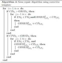
GeneRepair replaces the overlapped employees and, less and large task duration tasks, iteratively, with valid employees and tasks duration retrieved from a master individual template. Following algorithm-2 shows the generepair operator inserted as last oper-ations in loop. It also gives stoping criteria as schedule and cost margin.

Three different types of template can be used [24]:

1. Fixed template. This consist of a preset valid schedule (gener-ated by SGA), and remained constant throughout the generations. 2. Parent Template. Selected the fitter and elitist parent, and used that as the master template. This template varies for every individual corrected.

3. Random Template. For each corrected and valid individual a new template is generated, within the limitation of constraints of the SPSP.

Fig. 5. Gene Repair Genetic Algorithm

above the CPDTiand below the CDTi.

For first technique,if the GRODTiis higher than CPDTithen value of some alleles are changed to some lower value at random from 1 to 4. The alleles which are in between 5 to 8, are changed to 1 to 4 randomly and viceversa for value less than CDTi (Shown in Algorithm-3).

In second technique (Algorithm-4), the allele (value of gene) is changed according to the allele of corrective parent template. An algorithm-4 explains the scenario where the allele is changed to CPTiEj if it is less than and greater thanCPTiEj then and then only if task duration value GROD of task Tibelow the CDTi and above the CPDTi, respectively. ESTi∈TSTiis applied to schedule type-7 and type-8 only as it requires skill matching otherwise algorithm is without the condition of skill matching is used.

5. STUDY OF SCHEDULE TYPES 5.1 Implementation [37] [10] [9]

The code is written in JAVA using different GA classes in NET BEAN environment. The input parameters from input tables (Mentioned as INPUT in figs and tables )are taken as input to our Java code. The size of the population (number of different sets of parameter values considered for different schedule) is a user-defined variable. The default is 50. We get the various outputs which has been in the output tables and figures.

The initial population of chromosomes uses randomly-generated values for all the parameters (although optionally one can include an initial guess as one of the chromosomes). Each chromosome in the population is created by taking each input parameter value, and normalising it to a number between 0 and 1 with respect to its fitting range. Parameters cannot leave their fitting range. The chromosome is then simply the list of these values, and the population the list of all the chromosomes. The population is regularly stored to disk during a calculation, and can also be

Fig. 6. Gene repair Algorithm using random function

written on demand to facilitate restarting a run.

5.1.1 Evaluation of fitness. Genetic algorithms are normally maximising functions, so the fitness defined for each set of param-eter values is calculated as

N Ds=

GRDs maxi=1:SPGRDi

(12)

The above is the example given for only schedule type-2 but, the fitness formula changes as per the objective components change. Each time the fitness of a chromosome is better than the current notified by user and the parameter values are stored.

5.1.2 Selection of parents. The probability of a chromosome being selected as a parent for breeding purposes is linearly pro-portional to its rank by fitness as a fraction of the sum of the nor-malized objective components so better fitting parameters are more likely to be represented in the next generation. Selection is done by elitism method.

5.1.3 Breeding. Breeding,i.e.crossover is not always performed when creating children from selected parents a parameter Pc is defined which gives the breeding probability (default 0.85). If the parents are not bred, the children created are clones of the parents. Otherwise breeding occurs by taking the chromosome of each par-ent, listing the values as a single long string of numbers, choos-ing randomly a crosschoos-ing point, and swappchoos-ing all the digits after the crossing point from one chromosome to the other by crossover types.

5.1.4 Mutation. Each digit in each parameter value of the child chromosome is then assessed for mutation. The probability of mu-tation i.e. Pmis initially set to 0.01, but varies during the routine within the range between 0.01 and 0.05, increasing as the same fitness fitter chromosomes increases (and vice versa). If a digit is mutated, it is replaced with a random number (0-7).

5.1.5 Creation of new population. The above process is re-peated as many times as necessary to create a new population of chromosomes the same size as the initial population. With the elite option set (default) the fittest chromosome (best set of parameter values) is always preserved from one generation to the next, ensur-ing that the best fit never becomes worse (although worse fits are obviously still considered in each generation, and contribute to the exploration of parameter space). The new population then replaces the old, and a new generation begins.

5.2 Schedule Types and Discussions [37] [10] [9]

The final output of GA schedule is pool of chromosomes. Al-though we have got same fitness chromosomes, there are various genotypes individuals available for selection for the project man-agement.The project used in schedule is of 18 tasks, 10 employees, with the 5 skills.TT (Total Time) is considered as total efforts of the project is dependant on TT.

Following schedule types with their objectives and constraints are considered.

•Schedule Type 2(Only Total Time is considered).

•Schedule Type 2 (Hard Constraint:Task Comple-tion,objective:minimum CT ).

•Schedule Type 2(Objective:Minimum CT).

•Schedule Type 2 (Objective:Minimum GRD).

•Schedule Type 3(Objective:Minimum simple Cost).

•Schedule Type 3(Objective:Minimum simple ”Cost and Overtime as Penalty).

•Schedule Type 3 (Hard Constraint : Task completion).

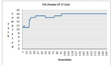
•Schedule Type 4 (Objective: Minimum cost and Total time).

•Other schedule types objectives and constraints are explained in respective section. The other schedules constraints and objectives can be seen in the respective graphs also. The hard constraints and objectives are the combination of schedule type-2 and type-3 and stopping criteria for these schedules is fitness and combination of CPI and SPI conditions ( as mentioned in the algorithm). Some figures, tables shows and respective schedule subsection gives the soft and hard constraints required for every contract-schedule types.

Following equation is applicable for every schedule plan and it is hard constraint except schedule-3Hard constraint is each and every employee must have at least one task assigned.

F or i= 1:n

z }| {

GRGADTi= e X

j=1

GRODTi,Ej ≥0 (13)

5.2.1 Schedule type1. This is not realistic. Objective is no re-striction on any triangular parameter and features. Schedule type1 only, for evaluation cause where the output gives its maximum level of 180 as the optimal solution the result shows increase in the as-signments of tasks as increase in the number of generations. This type of solution not feasible and not useful in real situation.

5.2.2 Fixed duration Schedule plan (schedule type 2). FDS plan requires the schedule of having minimum time, there is no restriction on cost,working load. This type of schedule can be done when PMs put restriction of negative float(slack) due to strict timed schedule. The hard constraint is fixed duration. All FTS must have all the skills required for the projects. Total float is strictly followed as all the activities and tasks are put on ASAP category. All PMP groups (IPG, PPG, EPG, CPG, MPG, CLPG) and their concerned employees included in this schedule type.

T F =P F+N F +F F (14)

where TF, PF, NF, FF are the Total float, positive float, negative float, free float respectively. Free float of every activity is kept, nearly, zero. Generally Crashing technique ( type of compression technique) is used. CPF(cost-plus fee) contract is suitable for this type of schedule.Nearly all activities are considered critical activity having zero float. Positive float is welcomed in this type of sched-ule. Each and every employee must have at least one task assigned. Hard Constraints are

1.

F or S= 1:s

z }| {

GRDS= n X i=1 e X j=1

GRSHDTi,Ej !

< CEDS (15)

Here, CED is expected duration but already fixed by contract. Gen-erally fixed duration is average duration calculated by an expert or COCOMO model.

3.

Hard Constraint

z }| {

GRODTi≤CDTi (16)

This type gives the project manager minimum level project execu-tion time with not having less constraints on project management it is a single variable objective function for optimization using ge-netic algorithm but the variable time is constant The schedule time or GRD is calculated additions of all the genes values as an Lan-grangs multiplier with devotion of employees, the objective of the function is to minimize time schedule only.

ScheduleM argin=CCTs−GRCTs CCTs

(17)

The proposed approach takes into account the task completion. The task completion definition is dependent on the COCOMO calcu-lated duration time CD. If contract is dependant on only on unit time i.e. milestones threshold time, it is up to the client and develop-ers trade off which is DUR (duration) deadline for each milestone. Some may take CD as threshold or EDUR or CPD. It is totally de-pendant on the time required to complete the project. Generally this type of contract only considers the time not the cost which comes under the ST-2. This type of schedule is the type of fixed duration where every task duration is decided. It is also called as contractual time or unit time contract. Even though, second importance is given to the cost as minimum objective. The TPG is kept in consideration for this type of schedule.

Another fixed duration type where task completion is hard con-straint and critical time is to be minimum. It is the combination of unit time and total time duration of the project. It is typical sched-ule where bonus or incentive in terms of leaves will be given. You can earn leave or take the cost in tern. This gives the free hands to the manager to select any person from team to fulfil the efforts of the activities, WBS component. Even though we are using TPG, the tasks can be completed by using parallel approach explicitly so that tasks can be completed below CED. BSD (Baseline start Date) and BFD (Baseline Finish Date) is strictly followed by only 10 PC margin.

Another type of schedule is schedule which takes into account only CT of project. This has got any hard constraint but objective is to have minimum CT. This type of schedule comes under only objective oriented optimisation.

Categorise of schedules are : Objective is minimum time

F Cs=

1 GRDs

(18)

Objective is minimum CT

F Cs=

1 CTs

(19)

Objective is minimum CT and Time penalty.

F Cs=

1 CTs

+ 1 T Ps

(20)

Objective is TT and Time penalty.

F Cs=

1 GRDs

+ 1 T Ps

(21)

Combination of above all:

F Cs=T C×(

1 CTs

+ 1 T Ps

) (22)

T Ps= (GRGADTi−CDTi)×η (23)

where

η=GRGADTi CDTi

(24)

Where,ηis penalty rate to be decided by PM.

5.2.3 Fixed budget Schedule (Schedule type 3). Schedule must be of minimum cost, there is no restriction on working load. Con-tract overrun is not allowed. This type of schedule involves Lump-Sum contract where total price is fixed at the time of contract. CPFF(cost-plus-fixed-fee) may be the total fixed cost also. CPI is used for the re-planning of this type of schedule as it plays vital role in AC (to be considered during the project). CV plays impor-tant role in re-planning also. DC is calculated as lump-sum amount. Some companies fix the lump-sum amount after the calculation of DC. This ST3 types of schedules gives chance to the mainly IPG, PPG as BAC has to be corrected in PPG

(DLCS) = n X i=1 e X j=1

GRSHDTi,Ej×SalEj !

< lump−sum

(25)

LSA=DCp=DLCS+M Cp+ECp+SCCp (26)

where p is the project to be estimated, S= 1:s, s: number of sched-ules.

Where DC⇒Direct Cost, DLC⇒Direct labour cost,MC⇒ Mate-rial Cost, EC⇒Equipment Cost,SCC⇒Sub-contract-cost. Salary of employee is excluding bonus, overtime, insurances and payroll taxes. Negative float activities are welcomed since as we can have time to do the project.

This schedule is of type which has minimum cost. This schedule type gives project manager as threshold in terms of money only. As project cost is hard constraint so that PM has to restrict him-self to complete the project within a proposed budget. The cost is depen-dent on the salary of the employee and ultimately and indirectly de-pends on the commitment of employee to the task. So, the schedule will be or may be showing the assignment to the employees which have the less salary. This type of schedule is useful only when we have more part time software professionals. Contract basis type of schedule comes under this category. We have two types schedule where the schedules can take two path. One is simple and only cost type schedule and second is genetic repaired cost type. First one tends to take the total cost into consideration and second one try to make to use as many as employees in the schedule. The second type schedule tries to complete the task as per proposed definition. First one takes the employee as many which has got the less salary but it happens partially in the second type. CPI is used as stopping criteria for the GRGA for both schedules.

F Cs=

1 DLCs

(27)

is using GRGA approach. Both types graphs for their fitness and cost verses generation has been shown in the figures it selves. The cost of using GA comes less than the GRGA as SGA does not take into account availability and task completion as per proposed ap-proach definition. Hence, the value GRGA cost comes more as it calculates the cost after making GR individuals in GA. The task completion for SGA ( as per Carl Chang (2001)) is ’Each task must be assigned at least one employee’. Our definition considers CO-COMO model’s CD as mentioned earlier. GR is dependent on the CD, that’s why GRGA cost is more than SGA.

1.

F Cs=

1 DLCs

+ 1 OTs

(28)

Above equation is optimisation of cost and over time as penalty. So the schedule will give the penalties if employees take the more time than the time required to complete the task. It means i.e. CPDTi ≥ GRGADTi ≥ CDTi. In other words, penalty will be given to the team. ( Here, OT is not the cost which gives more money while employee works more than his(r) capacity.)

OTs= (GRGADTi−CDTi)×µ (29) µis the rate of penalty and

µ=GRGADTi CDTi

×1.5. (30)

2.

F Cs=

1 CT DLCs

(31)

where, CTDLCs = TSM× GRCTsand TSM is team salary per month. GRCTsis the critical time obtained by proposed method. The above equation shows the fitness is dependant on the total salary. The total salary of the employee may be constant or may be varied according to the performance of the employee or em-ployees or team. The above schedule is dependant on critical time of the project. Ultimately, critical path is important and, decider of project cost. Typical tasks out of all tasks are given importance to complete the tasks in time. The task or the concurrent tasks should be completed within the limitations of CPM. This type of contract is dependant on the quality of the team and EMF of the team. As EMF for the team varies from 0.86 PC to 1.6 PC, the more money will be given to the less EMF team as this team contains quality of professionals. Some time, this type of contact may be dependant on the personal EMF factors defined by COCOMO-II.

3.

F Cs=T C×

1 CT DLCs

(32)

Another type of schedule gives importance to the time completion in terms of validation. Here, TC, Task Completed, is number of tasks satisfies the task completion criteria in GRGA. More weight will be given to the schedule as many as task satisfies this constraint. The objective is minimise the CTDLC.

F Cs=T C×(

1 CT DLCs

+ 1 OTs

) (33)

The above equation shows the minimisation of two objectives and satisfying TC as soft constraints. The stopping criteria of GRGA for all above schedule is fitness and CPI condition (mentioned in algorithm).

5.2.4 Fixed time-cost Based Plan (T&M type/Schedule type 4). Schedule and plan must be of minimum time and cost time. There is no restriction on working load. This type of schedule can be done when PM managers put restriction on negative floats not so strictly. All FTS must have all the skills required for the projects. Total float is not so strictly followed as all the activities and tasks are put on ASAP and ALAP category. The optimisation of all floating is done, ultimately tried to produce well floated sched-ule. CPIF(cost-plus-incentive-fee) contract is suitable for this type of schedule as this schedule is used for the comparison purpose with the others.Nearly all types of activities are considered. Criti-cal activity is used for Criti-calculation. This type of schedule involves BAC and CAC costs. SPI is used for the re-planning of this type of schedule as it involves SC during the project. SV plays important role in re-planning also. IPG do the tasks of initialisation and RE as PPG plan for the schedule but other group of EPG, CPG, MPG, CLPG professionals can be used to involve in the project groups to achieve the objective of this type of schedule

BACp=DCp+IDCp (34)

IDCp=AdminCostp+overheadp+Generalcostp (35)

where p is the project to be estimated. This type schedule shows optimization of time and cost. These two variables are in the same directions of the hypothesis where we should have minimum time and minimum cost. Whenever there is time limitation for the soft-ware related to the size of team and its productivity.

Fig. 8. Task Completion Vs Generation for Schedule Type 4(Objective: Minimum cost and Total time)

The formula in Equ.36 gives the most optimistic value of duration of every task but also that the duration of all the tasks required to complete the project. Though software project management allows one month per year or one month budget per year as margin that fulfils principle of management but, it also conflicts the total dura-tion of the project as relief in the scheduling problem.

5.2.5 Cost-plus-incentive-fee-contract plan( target schedule plan 5 ). Schedule must be of minimum time, cost,working load. Costing is related to incentives for the employees. The incentives are calculated on the basis of employees approach and other fac-tors of efficiency. Hard Constraint is duration of each task must be within limit.

CDTi≤GRGADTi≤CP DTi (36)

constraint is GRGADT iof each task Ti. Each Task duration must be in between CD and CPD. The cost estimator can get this type of schedule if he want to restrict each completion task duration within a range of optimistic to pessimisticEvery task must be completed within these two closed boundaries.CEVP process is adapted for this type of schedule. The objective function is the combination of cost, time, penalty and rewards. The reward or incentive is given accordingly if the task is in between likely and pessimistic in terms of money with a one and half rate of salary.

It is the type of combinatory problem of variable and constant con-straints, the schedule not only compromises time with the cost but also the individual task duration and employees salary. This type of schedule is a real schedule which considers the importance of the efforts calculated by the COCOMO model, the duration of this type of schedule gives a chance to reduce further time of duration by keeping optimistic task duration intact.

5.2.6 Unit prise/Cost Plus Schedule (Schedule type 6 ). This type of schedule can be done when PM managers want to do the study of optimistic, pessimistic and likely duration for effect on threshold parameters like cost drivers, time , quality factors, re-source values. All FTS must have all the skills required for the projects. SPI is used for the re-planning of this type of schedule as it involves SC during the project. SV plays important role in re-planning also. CAC is considered as cost of project. Total duration is hard constraint, here.

GRDs≤CT Ds (37)

The schedule type 6 considers minimum cost. Hard constraint is TC of the schedule. TC must satisfies the task completion criteria. This schedule comes under multiple objectives and single constraint mathematical problem where project manager has to restrict total average budget and total time.

The project manager has got the free hand to change the employee according to the bud-get and compensation to the time duration. Our solution in table-5 and table-6 gives the near optimal schedule which compromises mini-mum total duration and minimum cost by restricting the project duration in a total optimal duration. Above schedule type is dependant on the millstones and or each task. The millstones may be group of tasks to be performed as processes in one group. The SLDC is having analysis, design, im-plementation and testing phases, usually. Each phase may contain all the process groups mentioned depending on the requirement of the activity or umbrella activities in the project. Each process group is assigned to typical skilled employees which are dedicated to the specific and repeated type of work. Before starting of the project, all the milestones or targets are decided by WBS. The cost of the every unit millstone is decided which is put on the paper as per the table shown above. This cost is obligatory to the client to pay after the completion every unit part of the project.

This type of schedule is adapted when there is very small projects or the project which has not so high risk. In contrast to this also, some company gets the very large project and distribute the works in unit to the sub-companies and collect it after some millstones by making legal contract with others. The very large projects are also do this type of schedule where they want to distribute the risks into many domains and process groups. The advantage of the unit prise contract type of schedule is any one can from the huge numbers of team can understand the risks and communicate to the top management without hesitation and lowering the high risks to

the low risks by distributing the risks in the process groups.

Making the tiny parts of the huge project gives less responsibilities to the group to whom the unit is assigned with threshold date. This type of schedules require more management works than the actual work. This type of contract gives overhead to the management and management activities as this huge projet work has not only follow the TPG, but it has to follow the employee dependency also.

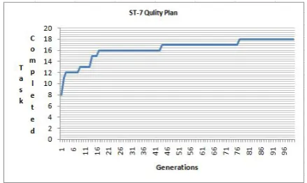
5.2.7 Quality schedule plan (Long Term business Plan) and schedule type 7. Nearly, all the parameters are considered as it required quality project to be delivered to the customer. Contract is all the combinations of subcontracts and contracts till we studied. There is no compromise with equality so the cost mostly includes the quality assurance and quality control related costs, hence the skill matching is must, here.

ESTi∈T STi (38)

The schedule type 7 considers skill matching and all objectives. Overloading is soft constraint.

This schedule is very important schedule to get a quality oriented project as skilled employee is only assigned to the task by consid-ering minimum salary and minimum time. These two variables are exactly opposite to the skill matching constraint as project manager doesnt have choice but to assign employee to the task considering strictly skill matching. This type of schedule surpasses minimum time and cost as skill matching restrictions increases the somewhat the cost and time in initial phase, but, after some duration we will get less time.actually. Fig.9 shows loading of employees in sched-ule type-7.

Fig. 10. Task completion Vs Generation for Schedule Type 7

Table 5. An Optimum Schedule type 6 ( Unit Prise )( objective:considering minimum cost, Hard constrained is Task completion).

T0 T1 T2 T3 T4 T5 T6 T7 T8

E0 1 0.5 1 0.75 0.75 0.5 0.5 0.75 0.5

E1 0.5 0.5 0.75 0.75 0.5 0.75 0.5 0.5 0.5

E2 0.5 1 1 1 1 1 0.75 0.75 1

E3 0.75 0.75 1 0.5 0.5 0.5 0.75 1 0.75

E4 0.5 1 0.5 0.5 0.5 0.75 0.5 0.5 1

E5 0.75 0.5 1 1 0.75 1 0.5 0.5 1

E6 0.75 0.75 0.75 0.75 1 0.75 0.5 0.5 1

E7 0.75 0.75 0.5 0.75 0.75 0.75 0.75 0.5 1

E8 0.5 0.5 0.75 0.5 1 0.75 0.75 0.75 0.5

E9 0.5 1 0.75 0.5 0.5 1 1 0.5 0.75

GRGD 6.5 7.25 8 7 7.25 7.75 6.5 6.25 8

T9 T10 T11 T12 T13 T14 T15 T16 T17

1 0.5 0.75 1 1 1 0.5 1 0.5 13.5

0.5 0.5 0.5 0.75 0.75 1 0.5 0.75 0.5 11

1 0.5 0.5 0.75 0.75 0.75 0.75 0.5 0.5 14

0.75 0.75 1 1 0.75 0.75 1 1 0.5 14

0.75 0.5 0.75 1 0.5 1 1 1 1 13.25

0.75 0.5 0.5 1 1 1 0.5 0.75 0.5 13.5

1 0.75 0.75 1 1 0.5 1 0.5 1 14.25

1 1 1 0.5 1 0.5 1 1 0.75 14.25

0.75 0.5 1 0.5 1 0.75 1 0.75 0.75 13

0.75 0.5 0.5 1 1 0.5 0.5 0.75 0.75 12.75

8.25 6 7.25 8.5 8.75 7.75 7.75 8 6.75 133.5

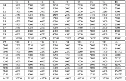
Table 6. An Optimum Schedule type 6 ( Unit Prise )( objective:considering minimum cost, Hard constrained is Task completion).

T0 T1 T2 T3 T4 T5 T6 T7 T8

E0 5000 2500 5000 3750 3750 2500 2500 3750 2500

E1 2000 2000 3000 3000 2000 3000 2000 2000 2000

E2 1500 3000 3000 3000 3000 3000 2250 2250 3000

E3 3750 3750 5000 2500 2500 2500 3750 5000 3750

E4 1500 3000 1500 1500 1500 2250 1500 1500 3000

E5 4500 3000 6000 6000 4500 6000 3000 3000 6000

E6 4500 4500 4500 4500 6000 4500 3000 3000 6000

E7 3750 3750 2500 3750 3750 3750 3750 2500 5000

E8 4000 4000 6000 4000 8000 6000 6000 6000 4000

E9 4500 9000 6750 4500 4500 9000 9000 4500 6750

UP 35000 38500 43250 36500 39500 42500 36750 33500 42000

T9 T10 T11 T12 T13 T14 T15 T16 T17 DC

5000 2500 3750 5000 5000 5000 2500 5000 2500 67500 2000 2000 2000 3000 3000 4000 2000 3000 2000 44000 3000 1500 1500 2250 2250 2250 2250 1500 1500 111500 3750 3750 5000 5000 3750 3750 5000 5000 2500 70000 2250 1500 2250 3000 1500 3000 3000 3000 3000 39750 4500 3000 3000 6000 6000 6000 3000 4500 3000 109750 6000 4500 4500 6000 6000 3000 6000 3000 6000 85500 5000 5000 5000 2500 5000 2500 5000 5000 3750 71250 6000 4000 8000 4000 8000 6000 8000 6000 6000 156750 6750 4500 4500 9000 9000 4500 4500 6750 6750 114750

44250 32250 39500 45750 49500 40000 41250 42750 37000 870750

respect to the high profile employees in management and technical fields. The skilled employee can be classified as per the five pro-cess groups mentioned earlier to do the specific tasks in the team. Team can be given name as per the process groups also. The main

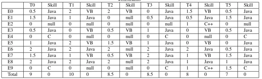
Table 7. An optimum Schedule 7: skill matching, all above objectives and constraints with overloading as soft constraint.

T0 Skill T1 Skill T2 Skill T3 Skill T4 Skill T5 Skill

E0 0.5 Java 2 VB 2 VB 0 Java 1.5 VB 0.5 Java

E1 1.5 Java 1 Java 0 null 0.5 Java 0.5 Java 1.5 Java

E2 0 null 0 null 0 null 0 null 1 C++ 0 null

E3 0.5 Java 0 VB 0.5 VB 1 Java 0 VB 0.5 Java

E4 0 C 0 null 0 null 0 C 0 null 0 C

E5 1 Java 2 VB 1.5 VB 1 Java 0 VB 0 Java

E6 2 Java 2 Java 2 null 2 Java 2 Java 0.5 Java

E7 1.5 Java 1 VB 0.5 VB 2 Java 1 VB 1.5 Java

E8 2 Java 2 Java 2 null 2 Java 1 Java 1 Java

E9 0 C 0 null 0 null 0 C 1 C++ 1.5 C

Total 9 0 10 0 8.5 0 8.5 0 8 0 7 0

Table 8. An optimum Schedule 7: skill matching, all above objectives and constraints with overloading as soft constraint. T6 Skill T7 Skill T8 Skill T9 Skill T10 Skill T11 Skill

E0 0 VB 0 null 2 VB 0 Java 0 null 1 Java

E1 0 null 1.5 C 1 Java 1 Java 2 C 1 Java

E2 1.5 C++ 0 null 0 null 0 Null 1 C++ 0 null

E3 2 VB 2 VC++ 0.5 VB 1 VC++ 0 null 1 VC++

E4 0 null 1 C 0 null 0 Null 1 C 0 null

E5 0 VB 0 null 1 VB 2 Java 2 C++ 1 Java

E6 0.5 C++ 0 null 2 Java 2 Java 0 C++ 0.5 Java

E7 2 VB 0 null 1 VB 0.5 Java 2 C++ 2 Java

E8 0 C++ 0 null 2 Java 1 Java 1 C++ 0 Java

E9 0 C++ 1 VC++ 0 null 0.5 VC++ 1 C++ 0.5 VC++

Total 6 0 5.5 0 9.5 0 8 0 10 0 7 0

5.2.8 Scope creeping plan / schedule type 8 /HRD plan. SCP plan requires the schedule of having minimum time and cost, and must follow working load. This type of schedule can be done when PM managers put restriction not only on quality but its feasible addition of features. Adding additional skilled employee, but not being given overload gives the scope creeping plan, but it gives another version of plan for the customers, also. Re-planning is the main purpose of this schedule as PM wants to add more and more skilled employee and gives various direction and scope of project. Finally, we gave same and equal weight age for the components of composite function.

This type of schedule considers minimum time and cost with overloading factor as hard constraint. Above all schedules may go beyond the overloading limit or capacity of particular employee. Above all schedule gives stress to the employee to complete within a total budget and total time without considering their speed and capability and stamina. But, this schedule type is another good example of optimization considering all the factors and assuming that every employee can do every task by limiting the overloading.

6. RESULT AND DISCUSSIONS 6.1 About graphs and Tables

Nearly all the schedule’s fitness vs Generation graphs are shown in Fig.12, 13, 16, 17 where we can see after some generation (after 100 approximately) fitness gets it’s steady positions. The fig.14 and fig.15 shows the graph of Time (Total Time) and Cost comparison with every schedules. But, critical time , GRGA CT time is given in the comparative table-11. Some schedules where

the task completion is necessary gives graphs on Task Completion VS Generation.

• TT is taken in the graphs in figures indicates the total time to require to complete the all the tasks(in sequence). TT is the additions of all the task duration which represent the total effort re-quires for the whole project. The TT doesn’t give the guarantee of completion task according to the definition of proposed approach for task completion.

•TC gives the critical time of the project for the particular schedule type. Even though TC is in the range of planned, it doesn’t give the assurance of completing the task in defined time. But, according to Carl’s definition of time completion that each task must have at least one employee. It results in increase in the percentage of task completion or nearly all tasks get completed. But, proposed approach implies tasks completion should have duration in defined rang.

Table 9. An optimum Schedule 7: skill matching, all above objectives and constraints with overloading as soft constraint. T12 Skill T13 Skill T14 Skill T15 Skill T16 Skill T17 Skill

E0 2 VB 0 null 2 VB 0 VB 0 null 2 Java

E1 0 null 0 null 0 Null 0 null 0 null 0.5 Java

E2 0 null 0.5 C++ 0 Null 1 C++ 1 C++ 0 C++

E3 2 VC++ 0.5 VC++ 1 VC++ 1 VB 1 VC++ 1.5 Java

E4 0 null 0 null 0 Null 0 null 0 nul l 0 null

E5 1 VB 1 C++ 2 VB 0.5 VB 0.5 C++ 2 Java

E6 0 null 2 C++ 0 Null 0 C++ 0.5 C++ 0.5 Java

E7 2 VB 2 C++ 2 VB 2 VB 2 C++ 1.5 Java

E8 0 null 1 C++ 0 Null 1.5 C++ 1.5 C++ 0.5 Java

E9 1.5 VC++ 2 VC++ 1.5 VC++ 1 C++ 1 VC++ 0 C++

8.5 0 9 0 8.5 0 7 0 7.5 0 8.5 0

Fig. 9. Employee loading and task duration for Schedule Type 7

number of tasks in the project. Other schedule gives less than 18 as TC is soft constraint.

GAGR behaves nearly same manner in all types of schedule resulted as this can be seen in fig.11. The curved lines are nearly

k to each others. Some tables in schedule’s sections gives the dedication of employees to the tasks ( (All output tables of every schedule is with the authors)). It shows various GRSHD with respect to the schedule types. Some tables in the study section gives value of GR duration in the range defined where TC is must.

6.2 Difference and similarities between ourANDCarl, Mark and Tao’s Approach [9]

Fig. 11. Linear behaviour of GRGA

Fig. 13. Fitness Vs Generation

Fig. 15. Cost comparison of all the schedules