A Macroeconomic perspective on skill
shortages and the skill premium in New
Zealand
Razzak, Weshah and Timmins, Jason
Department of Labour - New Zealand
8 February 2007
Online at
https://mpra.ub.uni-muenchen.de/1884/
A Macroeconomic perspective on skill shortages and the skill premium in New Zealand
W A Razzak and Jason Timmins† Department of Labour
Wellington / New Zealand
Abstract
Qualification and occupation-based measures of skilled labour are
constructed to explain the skill premium – the wage of skilled labour relative to unskilled labour in New Zealand. The data exhibit a more rapid growth in the supply of skilled labour than the skill premium, and a very large increase in the real minimum wage over the period from 1986 to 2005. We estimate the rate of increase in the relative demand for skills and the elasticity of
substitution. The data are consistent with skill shortages and a skill-bias technical change. We examine the effects of the minimum wage, capital complementarity, and the exchange rate on the skill premium. We also test whether the demand for skills and the elasticity of substitution varied across industries and over time.
Keyword: Skill-bias technical change, skill premium, the exchange rate JEL C23, J31, O3
†
The views expressed in this paper are ours and do not represent those of the Department of Labour. We thank Statistics New Zealand for the data. We thank Steve Stillman, Fiona Sterling, Jeff Borland, Niven Winchester and participants of the New Zealand Econometric Study Group at Otago University, 2006 for their suggestions. Contacts are
There is a large literature on wage inequality between skilled and unskilled labour. In the U.S., the skill premium – a ratio of the wage of skilled labour to the wage of unskilled labour – increased by more than 25 percent and the wage of unskilled labour declined over the period 1979-1995.i There is an agreement among economists that this wage inequality is explained by shifts in the supply of, and the demand for skills. However, there is a disagreement on the role played by the erosion of labour market institutions such the
minimum wage. And, there is a disagreement on whether the wage inequality reflected a secular rise in the demand for skilled labour, which is associated with the expansion in the use of computers (technology-skill
complementarity), and the decline in the relative supply of college equivalent workers, or it was a one-off episode.
To-date, there has been no empirical studies on this subject in New Zealand.ii The New Zealand government has been concerned about skill shortages (e.g., see the Department of Labour’s reports about skill shortages
information, skill news, and action plans among many other related documents).iii
New Zealand embarked on a very wide micro-macro reform process in the mid 1980s, which continued well into the early 1990s and undoubtedly affected the time series properties of the data. Also, the New Zealand data exhibited different trends from the US data. Wages of skilled and unskilled have positive mild trends. The distribution of the average hourly wage
exhibits small, but growing gaps, between those in the top (90th percentile), at the median and those who are in the bottom (10th percentile). By industry, the distribution shows positive trends in the 90th, 50th and the 10th percentiles, but the gaps between the skilled and the unskilled earners are negligible in almost all industries, except in industries like Finance, Insurance, Banking and
Community, which include the education sector and rely on computers. In these industries, the gaps between the top and bottom earners are relatively large and seem to be driving the aggregate data. Figure 1 plots the indices of the 90th, 50th and the 10th percentiles.
In the decade immediately after the reform from 1987 to 1996, the relative supply of skills grew rapidly (3.7 percent) while the skill premium declined (-1.2 percent), which is consistent with the prediction of economic theory. During the period from 1997 to 2005, the relative supply of skills grew at a positive, but a much slower rate (1.76 percent) and the skill premium
increased (1.5 percent). Most of the changes in the relative supply of skilled labour are induced by large changes in the supply of university-qualified workers with little or no significant changes in the supply of other
qualifications. Over the whole period from 1986 to 2005, the relative supply of skills increased by 2.7 percent and the skill premium increased only slightly (0.09 percent).
The shares of university-qualified workers, professionals and associate professionals etc. in total employment have been increasing over time, but they are relatively smaller than the shares of workers with high school, vocational and no qualifications. See figure 2. On average, less than 10 percent of employed workers have university training and professionals are less than 20 percent.
In this paper we will estimate the rate of change in the demand for skills and the elasticity of substitution. We also test the hypothesis that the small increase in the skill premium is related to the increase in the real minimum wage, which may have compressed the gap between the wage paid for skilled and unskilled labour. The real minimum wage increased by more than 20 percent over the period from 1987 to 2005.
Finally, the 1980s reform , the subsequent increased in the openness of the New Zealand economy and the floating of the currency in 1985 induced large swings in the real exchange rate (the index has a minimum value of 75 and a maximum value of 106). The share of exports in GDP increased from 23 percent in 1988 to 33 percent in 2005; the share of imports of capital goods such as machinery and plant increased from 3.5 percent in 2000 to 8.5 percent in 2005; the share of imported transport equipments and industrial increased from 0.35 percent in 2000 to 1 percent in 2005; and the share of imported intermediate inputs increased from 8 percent in 2000 to 11 percent in2005. Imported intermediate goods grew by 12 percent over this period.
The exchange rate affects labour demand and therefore wages via multiple channels. Campa and Goldberg (2001) provide a model and evidence that the labour demand curve, hence, wages are affected by the depreciation rate and that these changes come through changes in the shares of imports of intermediate inputs and the share of exports. We test the effect of the real exchange rate depreciation on the skill premium.
The analysis is organised as follows. First, we define “skilled labour”. In the literature, measures are mainly qualification-based, but in this paper we compute and analyse an occupation-based measure as well. Second, we estimate the rate of increase in the demand for skills. We take into account the effects of labour market institutions such as the minimum wage. Also, we take into account capital complementarities and examine the effect of the exchange rate depreciations on the skill premium. Third, we examine whether the demand for skilled labour has increased over time. Fourth, we examine whether skill shortages are an economy-wide phenomenon or whether they are localised in particular industries.iv
We estimated the increase in the demand for skills over the period 1987 to 2005 to be 2 percent. In the decade immediately after the reform from 1986-1996 the demand was about 1 percent. The demand for skills during the second decade after the reform from 1997 to 2005 is not significantly different from 2 percent, which is consistent with recent skill shortages. These
We estimated the elasticity of substitution to be >1. This evidence along with the increase in the demand for skills, the skill premium, and the supply of skills over time suggests that the increase in the demand for skills maybe consistent with a model of an endogenous skill-bias technical change, where technologies are skill-complementary, Acemoglu (1998).v An increase in the supply of skills induces firms to produce and / or adopt new technologies, which lowers the skill premium in the short run via the usual substitution effect. However, in the long run, the size of the market for technology could increase. If this effect dominates other relative price effects, the larger the supply of skills the larger is the technology effect. This direct technology effect induces higher profits, higher productivity, and higher skill premium. In the long run, these changes induce even more demand for skills.
Also, there is evidence for capital-skill complementarity. The minimum wage has a significant, but small economic impact on the skill premium. The exchange rate depreciation seems to reduce the skill premium.
Section 2 presents the theory. In sections 3 and 4 we discuss the data and test several hypotheses. In section 5 we introduce an occupation-based measure of skills and test the same hypotheses. Conclusions are in section 6.
2. Theory
We start with a typical Constant Elasticity of Substitution production function (CES) used in this literature, e.g., Autor et al. (2005), for aggregate output with two factor inputs; quantities of employed skilled and unskilled
labour, s
L and u
L , respectively. The superscriptssand udenote skilled and unskilled respectively. We will introduce industry and time subscripts later in this section.
(1) ρ ρ 1/ρ
] ) ( )
[(AsLs AuLu
Y = +
Output isY. The parameterρis a time-invariant production parameter. The skilled and unskilled augmenting technologies are s
A and u
A respectively.
Skill-neutral technological change raises s
A and u
A by the same proportion.
Skill-bias technical change involves an increase in s u
A
A / . The aggregate elasticity of substitution isσ =1/1−ρ.vi
In a competitive market, the marginal product of labour is equal to the real wage. Thus taking the derivative with respect to s
L equation (1) gives the wage of skilled labour:
(2) ρ ρ ρ ρ (1 ρ)/ρ
] )
/ ( [
/∂ = − + −
∂
= s s u s u s
s
A L
L A A L Y
Equation (2) implies that ∂ws /∂(Ls /Lu)<0so when the number of skilled workers increases relative to unskilled workers, their wage rate falls (i.e., excess supply).
Taking the derivative with respect to unskilled labour yields the wage of the unskilled labour:
(3) ρ ρ ρ ρ (1 ρ)/ρ
] ) / ( [ /∂ = + − ∂
= u u u s s u
u L L A A A L Y w >0,
Equation (3) implies ∂wu /∂(Ls /Lu)>0so that as the fraction of skilled labour in the labour force increases, the unskilled wage should increase.
Combining equations (2) and (3) we get the skill-premium, which is the ratio of the wage of the skilled labour to the wage of the unskilled (the marginal rate of substitution):
(4) σ σ σ
ρ ρ / 1 / ) 1 ( ) 1 ( − − − − = = u s u s u s u s u s L L A A L L A A w w
The ratio of wages (skilled to unskilled) is the wage premium, which can be re-written:
(5)
− − = u s u s u s L L A A w w ln 1 ln 1 ln σ σ σ
Equation (5) says the skill premium increases when we have skill shortages, i.e.,∂lnw/∂ln(Ls /Lu)=−1/σ, which is the usual substitution effect. For a given skill-bias of technology(As/Au), the relative demand curve for skilled labour is downward sloping with elasticity -1/σ .
If skilled and unskilled workers are producing the same good, but performing different tasks (e.g., complex and less complex), then an increase in the number of skilled workers will induce a substitution of unskilled workers with skilled workers because the skilled workers will be cheaper and can perform more complex tasks. However, if the skilled and unskilled workers produce two different goods, then the increase in the number of skilled workers will induce a substitution of the consumption of the unskilled good by the skilled workers.
Differentiating (5) with respect to technology gives:
Thus, the effect of a change in technology on the skill-premium depends on the size of the elasticity of substitution between skilled and unskilled labour. Ifσ is greater than one then improvements in the skill-complementary
technology will increase the skill premium. This is associated with an outward shift in the demand curve. Ifσ <1, an improvement in skill-complementary technology shifts the demand curve inward, reducing the skill-premium. However, it is understood that the skill premium (wage of the skilled labour) increases when workers become more productive and that is whenσ >1.
Acemoglu (2002) computes implied relative productivity for a given value of σ as
(7)
u s u s
u s
u s
L L L L
w w
A A
1 /
.
−
=
σ σ
This quantity is a proxy for skill-bias technological change. If s u
A
A / increases over time andσ >1 then this can be interpreted as a skill-bias technical
change, i.e., skilled workers are more productive.
In Acemoglu (1998), an increase in the relative supply of skills initially results in a decline in the skill premium (the substitution effect) along a downward slopping short-run relative demand for skills curve. Firms respond to the increase in the relative supply of skills by producing new technology, which is skill-complementary and the market size for technology begins to increase (the direct technology effect). The model predicts that if the direct technology effect dominates the relative price effect the skill premium increase because of the shift in the short-run relative demand for skills. The larger the supply of skills the higher the skill premium will be in the long run as firms’ profits and productivity continue to increase. The long-run relative demand for skills is upward slopping.
Figure 3 illustrates. The relative supply of skills is drawn with two segments, a vertical segment (infinitely inelastic supply) like in Acemoglu and a flatter upward slopping segment. The latter might be more consistent with the stylised facts presented earlier, i.e., New Zealand is a relatively low
productivity, low wage economy, and higher shares of unskilled workers such as no qualification (20 percent), high school and vocational qualifications (64 percent).
Let the initial relative supply of skills bes1 (solid line) and the initial short-run relative demand for skills bed1 (solid line). The demand intersects the supply
at point (a), which gives the skill premium s u
w
w1 / 1 . Now let the relative supply
of skills increase so the curves1shifts to the right tos2 (fainted line). The skill premium will start to decline along the downward slopping relative short-run demand curve to s u
w
w2 / 2at point (b). This is the substitution effect. Because
short-run relative demand for skills to shift up to eitherd2or d2′ (fainted lines).
Firms demand more skills to produce new technology. The first d2intersects the supplys2at point (c) while the second d2′intersects the more vertical
segment of the supply curve at point (c′). In both cases the skill premium increases, but s u
w
w3 / 3is a smaller increase than s u
w
w4/ 4. Point (c) describes the New Zealand data better than (c′) because the skill premium did not increase significantly even though the demand for skills increased
substantially and resulted in skill shortages.vii The long-run relative demand for skills connecting points (a) and (c′) isD′; it is upward slopping. The long-run relative demand for skills consistent with the New Zealand data isDand connects points (a) and (c).
The simplest regression to test for a trend in skill-bias technical change is given by the linear regression:
(8) t
A A
u t
s t
1 0
ln =δ +δ
In a regression like the one above, relative technological change depends on a constant term and time. If we substitute this in equation (5) we get:
(9) 1 ln( )
1 1
)
ln( 0 1 u
it s it u
it s it
L L t
w w
σ δ
σσ
δ
σσ− + − −
=
With the subscript (i) denotes industry and (t) denotes time. The assumption underlying this model is that the skill premium paid to a particular skill may vary across industries in the short run. Workers of similar skill levels move around, but in the long run the adjustment is complete and the skill premium equalize across industries. The assumption will be tested. We also assume that there is no a priori reason to believe that the elasticity of substitution is the same across industries. Pooling the time series and the cross section also increase the number of observations and allow us to estimate a more reliable standard errors.
Equation (9) is the “plain vanilla” version. It says that when ( / uit)
s it L
3. Data
We use pooled times series – cross section data from 1986 to 2005 for seven industries. The employment data used in this paper are from the New
Zealand Household Labour Force Survey (HLFS). For qualifications, the survey asks “What is your highest education level?” Respondents have several options, high school, vocational, university etc. The HLFS began in 1986. The last observation is September 2005. The HLFS samples
approximately 15,000 households and 30,000 individuals aged 15 and over each quarter. The HLFS did not begin collecting wage information until the introduction of an annual income supplement (HLFS-IS) to the June quarter HLFS in 1997. The wage data used between 1986 and 1996 are from the New Zealand Household Economic Survey (HES) and from 1997 to June 2005 are from the HLFS. The HES survey began in 1974 and was surveyed annually until 1998, and thereafter tri-annually. A sample of approximately 3,000 eligible households is achieved each year, divided equally between the four quarters.
Our sample also includes seven industries. (1) We combined Agriculture, Hunting, Forestry, Fishing, Mining and Quarrying in one to avoid missing values; (2) we combined Manufacturing, Electricity, Gas and Water for the same reason, (3) Construction, (4) Wholesale and Retail Trade, Restaurants and Hotels, (5) Transport, Storage and Communications, (6) Finance,
Insurance, Real Estate and Business Services, and (7) Community, Social and Personal Services. For simplicity, industry 1 will be referred to as Agriculture, 2 is Manufacturing, 4 Wholesale, 5 Transport, 6 Finance and 7 Community.ix
We use two measures for skills. The first is a qualification-based measure and the second is an occupation-based measure. The first measure is a widely used measure of human capital in this literature.x
We measure the relative supply of skilled labour as the ratio of employed workers with university qualifications plus ½ the employment of workers with school & vocational qualifications to employed workers with no qualifications plus ½ the employment of workers with school & vocational qualifications. Acemoglu (2002) and Autor et al. (1998), among others, use a similar
measure. The idea was first introduced by Welch (1969) to calculate college-equivalents. They aggregate non-college education groups, for example, those with some college and high school, into college-equivalents on the basis of the extent to which their wages track those of the pure skill groups.xi
4. Estimation
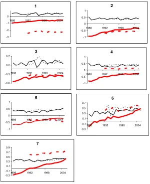
Figure 4 plots the data for ln( / itu)
s it w
w and ln( / uit)
s it L
L by industry. An obvious upward trend in the skill premiums in some, but not all industries, is apparent in the data. As shown earlier, relative average wages have not increased substantially over the sample. The skill premium data look almost identical whether we use a qualification or an occupation – based measure. Only in industry 6, Finance we observe significant differences. However, the relative supplies of skilled labour seem different in Agriculture, Wholesale, Finance and Community industries (1, 4, 6 and 7).
Our estimation strategy is as follows: Our sample includes 7 industries over the period 1986-2005. We provide a variety of fixed effect estimates. We begin by estimating the simple regression in equation (9), where the skill
premium is a function of a linear trend and the relative supply of skilled labour. We estimate the linear trend and the implied elasticity of substitution. We then augment the regression with one variable at a time; the minimum wage; the stock of capital per unit of output; output to account for the deviation from constant returns and variables that account for the business cycle; and a variable to capture the effects of international trade.
Most studies estimate a time series regression similar to that in equation (9) in levels. Surprisingly, although the data exhibit trend, tests for unit roots are not common in this literature. The individual industry level data have strong
positive trends, which might be stochastic. We used tests such as the ADF, Phillips-Perron (1987) and Elliott (1999) time series tests. We also ran a number of panel data unit root tests to take advantage of additional data points. We used the panel data version of the ADF, Im-Pesaran-Shin (1997), and Levin-Lin-Chu (2002), the Sarno-Taylor (1998) and Taylor-Sarno (1998). We could not reject the null hypothesis that the relative employment data have unit roots. For the relative wage of skilled labour, however, the tests were inconclusive. The tests are very sensitive to the lag structure. With one and two lags, most tests reject the unit root hypothesis. With three lags, the tests could not reject the unit root hypothesis. That being said, the coefficient estimates of the regression in levels can be super-consistent iff the variables are cointegrated.
It makes no sense to test for (no cointegration) if ln( / itu)
s it w
w is really I (0)
andln(Lsit /Luit)is I (1). However, when both time series are I (1) we also tested the residuals of equation (9) for unit root using the same tests above. We rejected the hypothesis of a unit root in the residuals, i.e., the two series are cointegrated. The interpretation of these tests is typical: unit root means shocks to relative employment and wages are persistent. We will run all regressions in levels following the literature, but we are cautious of the results in the absence of cointegration.
trend over the sample and estimates for trend and the elasticity of substation by industry. It is important to note that the HES wage data are more variable, compared with the HLFS-IS, and may reflect the smaller sample size of the HES, which has an implication for our estimated coefficients. We believe that the estimates over the sample 1997 onwards are much more reliable than estimates over the sample from 1987 to 1996 for this particular reason.
We use two estimators, EGLS and GMM-EGLS.xiii Table 1 reports 8 sets of estimates. In the first column we list the regressors. The wage premium and the relative supply of skills are qualification-based and measured as we
described earlier. In columns 2-3 we report the coefficient estimates and their P-values. The trend implies that demand for skills is 1.8 percent over the sample. The elasticity of substitution is 4 (1/0.25), which is very large
compared with estimates reported for the US in the studies we cited earlier.
In columns 4-5 we augment the regression with the log real minimum wage, which is only binding from 1992 onwards because industries paid higher wages than the minimum wage prior to 1992. We multiply the log real minimum wage by a dummy variable that takes a value of zero from 1986-1991 and 1 elsewhere. The coefficient is -0.02 and statistically significant. However, we interpret the magnitude as economically insignificant. The coefficient has the expected negative sign, i.e., an increase in the real minimum wage reduces the wage premium by a very tiny amount. The
inclusion of the minimum wage in the regression does not alter the estimate of the trend, which is 2 percent, but the elasticity of substitution increases, 4.3 (1/0.23).
Capital-skill complementarity was suggested by many, e.g., Griliches (1969) and Krusell et al. (2000). Economic theory predicts that industries with a larger stock of capital – given the amount of labour, have higher wages
because labour productivity would be higher. In columns 6-7 we augment the regression with two variables, capital stock intensity, which is measured as the stock of capital – real GDP ratio and the real GDP as an additional regressors, which captures the deviation from a constant return to scale (or the business cycle). The production exhibits constant returns to scale if this coefficient is zero. The elasticity of capital-GDP ratio with respect to the skill premium is 0.09 positive and only significant at the 10 percent level. GDP is insignificant. There is no change in the estimate of trend and the minimum wage. The trend is estimated to be 2.4 percent. The elasticity of substitution is 3.7 (1/0.27)
Campa and Goldberg (2001) present a dynamic model of labour market equilibrium, where within each year some combination of employment and wage adjustments equilibrate the labour market in response to shocks. They study the effect of the exchange rate on wages and employment. The
exchange rate shocks affect labour demand by affecting the marginal revenue product through changes in domestic and foreign sales and the cost of
imported intermediate inputs. They show that (i) when the production technology is labour-intensive, labour demand is less responsive to
markets raises the sensitivity of labour demand to the exchange rate; (iii) Higher export orientation of an industry increases the sensitivity of its labour demand to exchange rate movements; and (iv) Greater reliance on imported inputs into production reduces labour demand following a strong domestic currency. The New Zealand data show a very substantial growth in the imported capital goods in machinery and plant and in transport, 120 percent over the period from 2000 to 2006. The growth rate in imported intermediate goods is 12 percent over this period.xiv
In columns 8-9, we report a regression with the real exchange rate
depreciation rate as an additional explanatory variable. We also tried the nominal TWI exchange rate with no change in results. We don’t report the latter to save space, but the results are available upon request. The real exchange rate shock is∆lnqt, whereqtis the real exchange rate.
Depreciation of the Kiwi dollar has a negative sign, but insignificant. The trend is 1.6 percent, the elasticity of substitution is 3.4 (1/0.29). xv There is no significant change in the coefficient of the minimum wage. The coefficient of capital intensity increased slightly and remained significant. The coefficient of the real GDP is insignificant. The diagnostic tests of the regressions indicate that the fit is good and the residuals are white noise.xvi
The second set of results in table 1 are in columns 10-11, 12-13, 14-15 and 16-17 respectively. These regressions are estimated using GMM-EGLS. As shown, the parameter estimates of the trend are almost identical to those estimated by EGLS. However, the estimated elasticity of substitution changes significantly. We obtain estimates ranging between 1.58 and 3.57, which are within the reported US estimates. There is no change in the estimates of the coefficients of the minimum wage. The coefficient of capital intensity has become larger in size and more significant. The real depreciation is
significant and has a negative sign as predicted. In this particular regression the elasticity of substitution is 2.1 (1/0.47), the coefficient of GDP is larger, positive and significant at the 10 percent level, and the trend is significant but smaller in magnitude, 1 percent. The instruments used in GMM seem to have significant impact on the estimates, except for the estimates of the trend, which remain more or less unchanged. The diagnostic tests are unchanged from previous regressions. The over-identification restrictions of the
instruments could not be rejected by theJstatistics.
4.1 Did the demand for skilled labour change over time?
The answer is yes. Our time series sample is relatively short. Testing for change in demand over time requires splitting the sample into two sub-samples and testing whether the coefficients are equal. The dependent variable – the skill premium – consists of two different data sets, HES and HLFS. We split the sample at the end of 1996, where we ended the HES data and started the HLFS. Visually, there seems to be a clear positive trend in the skill premium from 1997 onwards, which is highly likely explained by the quality of the data. The hypothesis is that skill shortages intensified recently.
(10) it it i it u it s it u it s
it w a a td a td a L L u
w / )= + . + . + ln( / )+ψ ; ψ =ξ +
ln( 0 11 1 12 2 2 ,
Whered1is a dummy variable that takes a value of 1 from 1986 to 1996, and
zero elsewhere and d2is a dummy variable that takes a value of 1 from 1997 to 2005, and zero elsewhere.
We found: 99 . 0 94 . 1 89 . 0 : ) 014 . 0 ( ) 003 . 0 ( ) 06 . 0 ( ) 69 . 0 ( ) / ln( 44 . 0 . 016 . 0 . 01 . 0 04 . 0 ) / ln( 2 2 1 = − = = − + + = value p J DW R Stats Weighted L L d t d t w
wits itu sit uit
The increase in the demand in the first sub-sample is estimated to be 1 percent. Our original estimate of the increase in the demand for the whole sample was 2 percent. We test whether the estimate for the first sub-sample is equal to the estimate of the whole sample. The Wald statistic 2
1
χ has a P-value of 0.0137, thus the hypothesis is rejected. The estimate of the increase in the demand in the second sub-sample, however, is 1.6 percent, which is not different from 2 percent, i.e., the estimate of the whole sample. The Wald statistic has a p-value of 0.4480. We test whether the coefficients of the two sub-samples are equal. The p-values for the Wald statistics 2
1
χ is 0.0003. The hypothesis is rejected.
We interpret these results as evidence of the increase in the demand for skills in the period 1997 onwards. The increase in demand is consistent with the skill-bias technical change hypothesis.xvii However, we really don’t know how much of the result is attributed to the change in the surveys in 1997.
The results that the estimate ofσ is greater than one, the increase in demand for skills over time, and the increase in the supply of skills are consistent with “endogenous skill-biased technical change,” as we showed in the theory section. When skill-biased technologies are more profitable, firms will have more incentives to develop – and use or adopt – such technologies (e.g., the use of computers, Information Communication Technology ICT and General Purpose Technology GPT). This will lead to demand more skilled labour. Workers will also have incentives to up-skill so that they can use technologies.
4.2 Do the estimates of the demand and the elasticity of the relative supply of skilled labour (the implied elasticity of substitution) vary across industries?
The results are reported in table 2. One general conclusion is that the
coefficients vary across industries. And it is highly probable that the demand for skills is relatively higher in the services industries: Finance, Insurance, Real Estate and Business Service; Community, Social and Personal Services industries and in Transport, Storage and Communication.
We only report the EGLS results. GMM-EGLS is difficult to use in estimating this regression because of the large number of coefficients; we eventually run out of degrees-of-freedom. The first column reports the variables, followed by six columns. In the column labelled 1 we report the regression with varying trends. In the column labelled 2 we calculate the implied elasticity of
substitutionσ . All estimates of demand are positive and statistically
significant. The estimates seem to vary across industries. The hypothesis that all coefficients (γ1i’s) are equal is rejected.xviii The last three industries, namely, Transport; Finance …and the Community…, have the highest
estimated demand for skills, 1.6, 2.1 and 1.7 percent respectively. These two estimates are statistically not different from the averages reported in table 1 earlier.xix
In column 3 we report the results of the regression, where only the elasticity of the relative supply of skills varies across industries, while we kept the trend fixed. The estimated trend coefficient 0.014, which is again smaller than the average estimate reported in table 1 earlier. We found that the estimates of the elasticities also vary considerable across industries.xx The implied
elasticity of substitution reported in column 4 varies from 1.47 in Agriculture to 8.33 in Finance. The average is 3.32, which is higher than our earlier
estimates that we reported in table 1. We found that EGLS estimators in all regressions reported earlier, which we did not report, are also smaller in magnitudes than those of GMM-EGSL.
In column 5 we report the regression where all coefficients are allowed to vary across industries. There are more coefficients to estimate here and we
obviously run into degrees-of-freedom problems. The estimated standard errors are imprecise. The elasticities seem different from those reported in columns 3 and 4 thus one should be careful in interpreting them.
5. Another measure of skills
Some argue, correctly, that some occupations require skills, but not
necessarily a formal university education, e.g., a barber. There is very little use of occupation-based measures of skills in international literature. However, the New Zealand Department of Labour’s skill reports are only concerned with occupations. Similarly, Australia, the U.K. and the U.S. regularly publish statistics about occupational shortages.
classification in the1996/1997 HES survey. Third, some data are really unreliable because of small sample problem, e.g., female workers in Agriculture and Construction are very small samples. Also females in top professionals and managers are based on small samples.
To deal with these problems we had to use a much shorter sample. We use data from 1992, and effectively the samples are even smaller when we use GMM because the instruments are the lagged regressors. For this reason one should be cautious about these results. That being said, the results are qualitatively similar to those derived using qualification-based definitions earlier.
To see the differences between the surveys, for NZSCO68, we divide
individuals into three groups: Group 1 includes agricultural, production (and missing) workers and we call this group the unskilled labour. Group 2 includes clerical, sales, and services. Group 3 includes professionals and managers. For NZSCO90 group 1 includes agricultural, machine operators, elementary workers (and missing). Group 2 includes technicians, clerks, service/sales, and trade workers. Group 3 includes professionals and managers. We decided that group 3 is all skilled labour while group 1 is unskilled labour, but group 2 is half skilled and half is not.
The skill premium is measured as (group 3 wages + ½ group 2 wages) / (group 1 wages + ½ group 2 wages). Similarly, the relative skilled labour is measured as (employment of group 3 + ½ employment of group 2) /
(employment of group 1 + ½ employment of group 2).xxi
Over the period 1992-2005 and across all industries, average hourly wages for group 1, 2 and 3 grew by 2.3, 2.7 and 3.4 percent respectively.
Employment grew by 2.6, 2.0 and 3.7 percent respectively. The wage premium grew by 0.07 percent on average while the relative skilled
employment grew by 0.05 percent. These means suggest that demand must have shifted up, slightly, more than supply.
The main GMM-EGLS regression results (effective sample 1996-2005) are given by: (11) 99 . 0 72 . 1 96 . 0 : ) 0654 . 0 ( ) 0000 . 0 ( ) 0077 . 0 ( ) / ln( 34 . 0 008 . 0 19 . 0 ) / ln(
2 = = − =
− + = value p J DW R Stats Weighted L L t w
wits itu sit uit
We used a constant term, a trend term and four lags of ln(Lsit /Luit)as
because we have a smaller sample and we wanted to conserve on the degrees-of-freedom.
We have data for arrivals and departures by occupation only. We don’t have data by industry so we could not include such variable in the regressions. Workers of various skills leave New Zealand for many reasons, which reduce the supply of skills and affect the skill premium. Over the period from 1992 to-date, New Zealand annual net migration (arrivals minus departures) has been positive from 1992-1998, negative from 1998-2000, and positive since 2001. Some occupations still have a negative net migration. However, net migration for “top guys” the managers, professionals, technicians and associate
professionals has been positive since 2002.
6. Summary and Conclusions
The New Zealand economy has been experiencing a strong upward shift in the demand for skilled labour and a significant equal increase in the supply of skilled workers which are consistent with an endogenous skill-bias technical change. Firms’ adoption of new technologies requires skilled labour, which increases the demand and induces workers to up-skill, which increase the supply. Our estimates of the elasticity of substitution exceed one, thus given these demand and supply changes, improvement in the skill-complementary technology increased wages for skilled and unskilled labour. However, the increases in the wages were small because the increase in the demand was only slightly larger than the increase in the supply of skills. Using qualification-based measures of skilled labour, our estimates of demand are about 2 percent annually over the period from 1986 to 2005.
We found significant differences across industries when we allowed the coefficient to vary across industries. Our estimates of the elasticity of substitution varied across industries. Also, demand for skills are relatively higher in the services industries (i.e., Finance, Insurance, Real Estate, and Business Services and Community, Social and Personal Services), which are more dependent on computers and ICT. We conclude that the services industries may have experienced high levels of complementary technological shocks and accounts for more skill shortages. Relative to Agriculture and Manufacturing, these industries’ GDP still makes a small percentage of total GDP, but the OECD trend of these industries seems to increase over time and one can imagine that the size of this sector in New Zealand to increase in the future. This will mean more demand for skilled labour. There is an increase in demand for skilled labour across all industries from1997 onwards as compared with the demand over the period prior to 1997.
We attempted to test the effect of openness of the economy on the demand for labour and the skill premium by using the real depreciation rate (the relative price of non tradable goods) as an additional regressor, Campa and Goldberg (2001). The idea is that the orientation of the economy changed in 1985 when the exchange rate was floated and its variability increased
significantly. We are cautious about our results because they seem to be sensitive to the method of estimation. However, the sign of the estimated coefficient is negative as predicted by the theory. We interpreted this to mean that the real depreciation of the Kiwi dollar increases the cost of imported intermediate inputs, thus higher cost of production. The depreciation also increases the revenues generated by exporting industries. On average, if the cost exceeds the revenues the demand for skilled labour and the skill
References
Acemoglu, D., “Why Do New Technologies Complement Skills? Directed Technical Change and Wage Inequality,” Quarterly Journal of Economics, 113 (November), 1998, 1055-1089.
Acemoglu, D., “Human Capital Policies and the Distribution of Income: A Framework for Analysis and Literature Review,” New Zealand Treasury Working Paper 01/03, 2001.
Acemoglu, D., “Technical Change, Inequality and the Labor Market,” Journal of Economic Literature, Vol. XL (March), 2002, 7-72.
Autor, D., L. Katz and M. S. Kearney, “Trends in U.S. Wage Inequality: Re-Assessing the Revisionists,” NBER Working Paper No. 11627, 2005.
Autor, D., L. Katz and A.B. Krueger, “Computing Inequality: Have Computers Changed the Labor Market?” The Quarterly Journal of Economics, 1998, 1169-1213.
Beaudry, P. and D. Green, “Changes in U.S. Wages 1976-2000 Ongoing Skill Bias or Major Technological Change?” Journal of Labor Economics, Vol. 3 No. 3, 2005, 609-648.
Berman, P., J. Bond and S. Machin, “Implications of Skill- Biased Technological Change: International Evidence,” Quarterly Journal of Economics 118 (November), 1245-1279, 1998.
Borland, J., “Economic Explanations of Earnings Distribution, Trends in the International Literature and Application to New Zealand,” New Zealand Treasury Working Paper 00/16, 2000.
Campa, J. M. and S. L. Goldberg, “Employment Versus Wage Adjustment and the U.S. Dollar,” Review of Economics and Statistics August 1, 2001, V (83), 477-490.
Card, D. and T. Lemieux, “Can Falling Supply Explain the Rising Return to College for Young Men?” The Quarterly Journal of Economics 116 (May) 2001, 705-46.
Elliott G., (1999) Efficient Tests for Unit Root When the Initial Observation is Drawn from its Unconditional Distribution, International Economic Review 140:3, 767-783.
Engelbrecht, H-J and V. Xayavong, “ICT intensity and New Zealand’s productivity malaise: Is the glass half empy or half full?” Information Economics and Policy 18, 2006, 24-42.
Consequences of Increasing Income Inequality, Chicago: University of Chicago Press, 2001, 37-82.
Griliches, Z., “Capital-Skill Complementarity,” The Review of Economics and Statistics 51, 1969, 465-468.
Hyslop, D., Dave Maré and Jason Timmins, "Qualifications, Employment and the Value of Human Capital 1986-2001", New Zealand Treasury Working Paper 03/35, 2003.
Im, K. S., M. H. Pesaran, and Y. Shin, (1997), Dept Applied Economics Cambridge DP Dec 1997
(http://www.econ.cam.ac.uk/faculty/pesaran/lm.pdf)
Johnson, R., W. A. Razzak and S. Stillman, “Has New Zealand Benefited from Its Investments in Research and Development?” Forthcoming Applied Economics 2006.
Lemieux, T., “Decomposing Residual Wage Inequality: Composition Effects, Noisy Data, or Rising Demand for Skills,” University of British Colombia, 2001.
Katz, L. and K. Murphy, “Changes in Relative Wages 1963-87: Supply and Demand Factors” The Quarterly Journal of Economics 107 (February) 1992, 35-78.
Katz, L. and H. Autor, “Changes in Wage Structure and Earnings Inequality,” In O. Ashenfelter and D. Cards, eds. Handbook for Labour Economics, North Holland, Vol. 3, 999.
Krusell, P., L. E. Ohanian, Jose-Victor Rios-Rull, G. L. Violante,” Capital - Skill Complementarity and Inequality: A Macroeconomic Analysis,”
Econometrica, Vol. 68, No. 5 (September) 2000, 1029-1053
Knuckey, S., H. Johnston, C. Campbell-Hunt, K. Carlaw, L. Corbett and C. Massey, “Firm Foundations: A study of New Zealand business practices and performance,” Ministry of Economic Development, 2002.
Levin, A., C. F. Lin and C. S. Chu, “Unit Root Tests in Panel Data:
Asymptotic and Finite Sample Properties,” Journal of Econometrics 2002 108, 1-24.
Machin, S. and J. van Reenen, “Technology and Changes in Skill Structure: Evidence from Seven OECD Countries,” Quarterly Journal of Economics, 113 (November), 1215-1244, 1998.
Phillips, P. C. B., “Time Series Regression with a Unit Root,” Econometrica 1987, 55, 277-301.
Razzak, W. A., “Towards Building A New Consensus AboutNew Zealand’s Productivity,” Labour Market Policy Group Occasional Paper, Wellington, New Zealand, 2003.
Sarno, L. and M. Taylor, “Real Exchange Rates Under the Current Float: Unequivocal Evidence of Mean Reversion,” Economics Letters 1998, 60, 131-137.
Table 1: Panel EGLS and GMM-EGLS regressions with cross-section weights and white cross-section standard errors and covariance – degree-of-freedom correction
it t it
it it
t u
it s it u
it s
it w a at a L L a w a Y a K Y q
w / )= + + ln( / )+ min + ln( )+ ln( / )+ln∆ +ψ
ln( 0 1 2 3 4 5 ; ψit =ξi +uit.
EGLS 1987-2005 GMM-EGLS 1990-2005
1 2 3 4 5 6 7 8 9 10 11 12 13 14 15 16 17
Coef. Pvalue Coef. Pvalue Coef. Pvalue Coef. Pvalue Coef. Pvalue Coef
.
Pvalue Coef. Pvalue Coef. Pvalue
t 0.013 0.0000 0.016 0.0000 0.01 0.0608 0.003 0.5472 0.02 0.0004 0.02 0.0002 0.020 0.0059 0.010 0.2363
) / ln( uit
s it L
L 2 -0.29 0.0000 -0.20 0.0177 -0.19 0.0337 -0.19 0.0269 -0.59 0.0007 -0.30 0.0729 -0.39 0.0560 -0.47 0.0188
t
w
min ln
x
dummy3
- - -0.03 0.0000 -0.03 0.0000 -0.03 0.0000 - - -0.03 0.0014 -0.03 0.0000 -0.02 0.0026
) / ln(Kit Yit
4
- - - - 0.06 0.0479 0.06 0.0448 - - - - 0.11 0.1349 0.13 0.0824
it
Y
ln 5 - - - - 0.18 0.0865 0.38 0.0017 - - - - -0.008 0.9651 0.36 0.1062
t
q
∆
ln 6 - - - -0.14 0.0117 - - - -0.13 0.0217
Weighted Stats
2
R 0.86 0.92 0.90 0.91 0.84 0.90 0.93 0.91
DW 1.75 1.84 1.87 1.91 1.92 1.96 2.0 2.0
JP-value - - - 0.98 9.99 0.99 0.99
1. The skill premium wits/wituis measured by average hourly wages for full time employed workers with university qualifications plus ½ the wage of workers with school & vocational qualifications as a ratio to the hourly wage of workers with no qualifications plus ½ the wage of workers with school & vocational qualifications.
2. The relative supply of skilled labour uit s it L
L / is measured by employed workers with university qualifications plus ½ employed workers with school & vocational qualifications. Unskilled labour is measured by employed workers with no qualifications employed workers with school & vocational qualifications.
3. Minimum wage is real deflated by the CPI. The variable includes a dummy variable to control for the period before 1992, where it was not binding because industries paid higher than the minimum wage.
4.Kit is the stock of capital. 5. Yitis real GDP. 6. qtis the real exchange rate.
Industries are: (1) Agriculture, Hunting, Forestry, Fishing, Mining and Quarrying, (2) Manufacturing, Electricity, Gas and Water, (3) Construction, (4) Wholesale and Retail Trade, Restaurants and Hotels, (5) Transport, Storage and Communications, (6) Finance, Insurance, Real Estate and Business Services, (7) Community, Social and Personal Services.
Table 2: Panel EGLS regressions with section weights and white cross-section standard errors and covariance – degree-of-freedom correction
it i it it u it s it u it s it u v L L t w w + = + − +
=γ γ γ ln( ) ε ε
)
ln( 0 1 2 . The sample is 1986-2005.
1 2 3 4 5 6
coefficient σ coefficient σ coefficient σ
0 γ 0.07 (0.2270) 0.02 (0.7498) 0.01 (0.8829) ) /
ln( uit
s it L
L by industry γ2 -0.37
(0.0005)
2.70 -
Industry 1 - -0.68
(0.0006)
1.47 -0.85
(0.1001)
1.17
Industry 2 - -0.37
(0.0038)
2.70 0.07
(0.7295) -
Industry 3 - -0.43
(0.0562)
2.32 -0.28
(0.4649) -
Industry 4 - -0.52
(0.0004)
1.92 -0.43
(0.1050)
2.32
Industry 5 - -0.32
(0.0060)
3.12 -0.92
(0.0009)
1.08
Industry 6 - -0.12
(0.3086)
8.33 -0.08
(0.7441) -
Industry 7 - -0.29
(0.0004)
3.44 -0.58
(0.0133)
1.72
Trend by Industry γ1 0.014
(0.0000)
- - -
Industry 1 0.007
(0.0620)
- - 0.018
(0.1151)
Industry 2 0.012
(0.0006)
- - -0.00
(0.7362)
Industry 3 0.012
(0.0000)
- - 0.011
(0.1215)
Industry 4 0.009
(0.0091)
- - 0.01
(0.1560)
Industry 5 0.016
(0.0000)
- - 0.032
(0.0000)
Industry 6 0.021
(0.0000)
- - 0.013
(0.1060)
Industry 7 0.017
(0.0000)
- - 0.024
(0.0031) Weighted stats
2
R 0.90 0.88 0.89
DW 1.97 1.97 2.06
. .e
S 0.08 0.08 0.08
Figure 1: Index Wages
1
1.5
2
2.5
19
86
19
87
19
88
19
89
19
90
19
91
19
92
19
93
19
94
19
95
19
96
19
97
19
98
19
99
20
00
20
01
20
02
20
03
20
04
20
05
Figure 2: Shares in employment. No qualification: Solid thick line; School qualification: Solid thin line; Vocational qualification: Dashed solid line; University qualification: Dotted thin line
I nd ust r y 1
0 0.1 0.2 0.3 0.4 0.5 0.6
1986 1992 1998 2004
I nd ust r y 2
0 0.2 0.4 0.6
1986 1992 1998 2004
I nd ust r y 3
0 0.1 0.2 0.3 0.4
1986 1992 1998 2004
I n d u st r y 4
0 0.1 0.2 0.3 0.4 0.5
1986 1992 1998 2004
I n d u st r y 5
0 0.2 0.4 0.6
1986 1992 1998 2004
I n d u st r y 6
0 0.2 0.4 0.6
1986 1992 1998 2004
I n d u st r y 7
0 0.2 0.4 0.6
1986 1992 1998 2004
(1) Agriculture, Hunting, Forestry, Fishing, Mining and Quarrying, (2) Manufacturing, Electricity, Gas and Water,
(3) Construction,
(4) Wholesale and Retail Trade, Restaurants and Hotels, (5) Transport, Storage and Communications,
Figure 3:
Endogenous Skill-Bias Technical Change and the Dynamic of the Skill Premium
c
c′
u s
w w a) 1 / 1
(
u s
w w b) 2/ 2
(
u s
w w c) 3 / 3
(
u s
w w
c) 4 / 4
( ′
u s
L L /
1
s s2
1
d
2
d′
D′
2
d
D
b
Figure 4: Solid lines are qualification-based measures. Dotted lines are occupation-based measures. Thin lines areln( / itu)
s it w
w . Thick areln( / uit)
s it L
L .For
qualification-based measures the sample is 1986-2005. For occupation-based measures the sample is 1992-2005.
1
-3 -2 - 1 0
1986 1992 1998 2004
2
- 1 - 0.5 0 0.5 1
1986 1992 1998 2004
3
- 0.8 - 0.3 0.2 0.7
1986 1992 1998 2004
4
-1 - 0.5 0 0.5 1
1986 1992 1998 2004
5
-1 - 0.5 0 0.5 1
1986 1992 1998 2004
6
- 0.3 - 0.1 0.1 0.3 0.5 0.7
1986 1992 1998 2004
7
- 0.3 - 0.1 0.1 0.3 0.5 0.7 0.9
1986 1992 1998 2004
(1) Agriculture, Hunting, Forestry, Fishing, Mining and Quarrying, (2) Manufacturing, Electricity, Gas and Water,
(3) Construction,
(4) Wholesale and Retail Trade, Restaurants and Hotels, (5) Transport, Storage and Communications,
i For the U.S. for example see Katz and Murphy (1992), Murphy and Welch (1992), Katz and
Autor (1999), Katz and Autor (1999), Goldin and Katz (2001), Acemoglu (1998), Acemoglu (2002), Lemieux (2002), Card and Lemieux (2001) among others. International studies includes, for example, Berman, Bound and Machin (1998), and Machin and Van Reenan (1998).
ii
The New Zealand Treasury published two discussion papers, Borland (2000) and Acemoglu (2001) about the macroeconomic perspective of skill shortages, but neither one provided empirical analysis of the New Zealand data.
iii
The Department of Labour uses economy-wide information about aggregate quantities of particular types of skills (The New Zealand Institute of Economic Research Quarterly Survey of Business Opinion – QSBO and Statistics New Zealand’s Quarterly Employment Survey – QES, and sector-specific information (sources are Skill NZ, Career Services, DWI and the Ministry of Education).
iv
We could not test for male and female separately because female data have missing values for example in industries like Agriculture and Construction. There are more missing data when examine qualification. For example female university-qualified workers are difficult to find in Agriculture and Construction. Removing these industries reduce the sample and cause serious estimation difficulties. Also, we could not test whether workers with different experiences have different demand profiles and elasticity of substitution because of (1) lack of data to measure experience and (2) when using age as a proxy for experience we
encountered missing data for young and old people with university degrees, which forced us to work with very small sample. Also we found missing data for age in industries like Agriculture, Fishery…and Construction, which reduces the size of the panel and makes the estimates of the standard errors large.
v
Knuckey, S. et al. (2002) is a Ministry of Economic Development report, which provide anecdotal evidence on the positive trend in the expenditures on computers and other Information Communication Technology in New Zealand since 1996.
vi
The production function allows for different interpretations. It is consistent with a closed economy with an underlying utility function defined over two goods, one is produced by skilled labour and the other is produced by an unskilled labour. It is also consistent with a one-good economy, where skilled and unskilled workers are imperfect substitutes in the production of this good. Further, it is also consistent with an economy with different sectors producing goods that are imperfect substitutes and skilled and unskilled workers working in these
sectors. Skilled and unskilled labour are gross substitutes whenσ >1and gross complements
whenσ <1. σ →0is the case, where output could be produced by fixed proportions
(Leontieff); σ →∞, is where skilled and unskilled workers are perfect substitutes; and when
1
→
σ the production function is a Cobb-Douglas.
vii
Future research will be to estimate the labour supply elasticities.
viii
The technology shocksAsandAuare unobservable. We have data for TFP by industry, but
these cannot be specified in terms of skilled and unskilled labour so we cannot use TFP data in the regressions. It is common in this literature to use a time trend. It is also difficult to estimate the effect of computers and ICT because the data by industry are not adequate for estimation. The sample is too small (1996 onward at most).
ix
x
It was not possible to intersect qualification and occupation because of small sample size in the data. For example, it is difficult to find data for professionals and managers with no qualifications and Agricultural workers with university degrees…etc.
xi
We tried a sensitivity analysis by using weights like ¼ and ¾ instead of ½, but they made very little difference.
xii
We dropped this measure. The regression result has incorrect signs. The regression is
misspecified due to measurement errors.
xiii
The Generalized Least Squares method and the Generalized Method of Moments are used to estimate the coefficients. Dropping the subscripts for simplicity, the GMM estimator
minimises S(β)=(
∑
h′ψ(β))′W(∑
h′ψ(β))=g(β)′Wg(β)with respect toβ for a chosen pxpweighting matrix W, where g(β)=
∑
g(β)=∑
h′ψ(β) and his a Txpmatrix of instruments.GMM accounts for endogeneity. The former estimator produces biased and inconsistent parameter estimates if any of the regressors are endogenous. It is also appropriate when the economic model is not fully specified. GMM is a robust estimator because it does not require information about the exact distribution of the error term. A common and typical problem with GMM is the weak and inadequate instruments. Unfortunately, we only have lagged values of the regressors, the trend, and a constant term to use as instruments. We use up to three lagged values of the regressors as instruments unless otherwise indicated.
xiv
They also show that industry-specific elasticity of response to the exchange rate
movements are significantly correlated with the skill composition of workers. Industries with a higher proportion of college-educated workers exhibit higher wage elasticities in response to the exchange rate shock, possibly because of the high cost of hiring or firing workers.
xv
We also allowed the real exchange rate depreciation to vary across industries. We
estimated the regression using EGLS only. We found that the real depreciation rate to have a negative effect on the skill premium in all industries, except Agriculture. For Agriculture the coefficient was positive and larger in magnitude than all other coefficients, 0.47. Agriculture is an unambiguously export-oriented industry in New Zealand so it must be highly affected by fluctuations in the real exchange rate. Most significant coefficients are found in Community and Wholesale. The rest of the coefficients are either marginally significant or insignificant. Results are available upon request.
xvi
The weightedR2are between 0.84 and 0.93;DWstatistic is between 1.92 and 2.0 so we
cannot reject the hypothesis that the residuals are white noise since we have already
corrected the regressions for heteroscedacticity, and theJstatistics for testing the
over-identifying restrictions suggest that the hypothesis of over-over-identifying restrictions cannot be rejected in all regressions.
xvii
We tested the hypothesis that demand is the same over the sample 1986-1992, and 1993-2005. We could not reject the hypothesis that they are equal. The estimated demand was 2 percent per annum.
xviii
The Wald test is distributedχ62and the p-value is 0.0000
xix Subsets of the estimates are equal. Manufacturing and Construction have the same
estimates of demand; the Waldχ12 p-value is 0.9639 so we cannot reject the hypothesis that
estimates. The Waldχ12p-value is 0.7753. Similarly Transport and Community, Social and
Personal Services have similar demand estimates, where the Waldχ12p-value is 0.8977.
xx
TheH0:coefficients are equal. The Wald statistic is
2 6
χ and has a P-value of 0.0001.
xxi