Design and Development of GUI for Magnetic Suspension Reaction Wheel

Technology (IJRASET)

©IJRASET 2015: All Rights are Reserved

151

Design and Development of GUI for Magnetic

Suspension Reaction Wheel

Lekshmi Nair. G1, Mr. Sanoop. M.K2, Mr. Haridas. T.R3 , Mrs. Isabel. R.A4, Miss. Divya. C.M5 1

Student, ME, SCET, Manivila, 2Sci/Eng-D, ISRO Inertial Systems Unit Trivandrum 3

Sci/Eng-G, ISRO Inertial Systems Unit Trivandrum 4&5Assistant Professor, Sivaji College Of Engineering & Technology, Manivila, KK Dist.

Abstract- This paper focuses on the design and development of a Graphical User Interface system (GUI) for the performance analysis of the Magnetic Suspension Reaction Wheel (MSRW) with four degrees of freedom. The GUI development is based on the detailed mathematical analysis of MSRW which includes the principle of active suspension, dynamics of the rigid rotor, and controlling of the rigid rotor. The developed system is flexible to be applied for both the linear and non-linear models as well as have a provision to check for the dynamic characteristics of individual degrees of freedom and four degrees of freedom. The developed system model using Matlab Software based on the mathematical analysis features interactive environment by inputting the basic system parameters.

Index Terms- Graphical User Interface system (GUI), Magnetic Suspension reaction wheel (MSRW), reaction wheel Assembly (RWA)

I. INTRODUCTION

The reaction wheel Assembly (RWA) consists of a rotating flywheel mounted on a shaft, supported by bearings and driven by a brushless DC motor [2]. Conventional system uses lubrication (oil etc) for the free movement of the rotor with minimum loss. The magnetic suspension system features Active Magnetic Bearings (AMB) which accounts for no lubrication, no stiction, longer life, high reliability and higher rotational speed. The paper is organized as follows:

II. AMBSYSTEM

A simple AMB system with one degree of freedom consists of a rotor, bearing, sensor, controller and power amplifier. The control of the system is achieved by using a feedback loop. The rotor position determines the stability and reliability of the system which can be controlled by control current.

U.J.Bichler[1] simulated and compared the different possibilities of active vibration suppression in low noise magnetic bearing reaction wheel. The study of the effect created by the micro-vibrations in wheel assembly on the performance of sensitive payloads was studied in [2]. [3] describes a comparative analysis using simulation for over the advantages of state-space control method in the magnetic bearings and digital PID control. The superiority of nonlinear controllers over conventional controllers for systems with large variations in operating point via experiment is described in [4]. The dynamic modelling of Magnetic Levitation System with the linear controllers linearized around a equilibrium point as well as with the nonlinear state space controllers based on feedback linearization is presented in [5]. In [6] the author carried out research on the development of a magnetically suspended momentum wheel capable of actively reducing imbalance vibrations by focussing on the implications on feedback control design. To ensure an easy way of tuning parameters with good damping environment, Ritonja[7] presented a rule-based method for designing PID controllers for active magnetic bearings .

By giving the electromagnetic forces, the suspension of the rotor can be achieved [8]. Thus by providing control current though the bearing; electromagnetic force can be generated and the suspension system can be controlled. The feedback structure comprises of rotor, bearing, sensor, controller and amplifier. This model can be extended up to five degrees of freedom system for which the rotor can be controller in its five axises.

Technology (IJRASET)

©IJRASET 2015: All Rights are Reserved

152

In some of the applications, magnetic suspension systems need to operate over large variations in air gap. Hence nonlinearities which may occur during the operation of the system will affect the performance. Also due to theses nonlinear effects, it is difficult to design a controller which is reliable and also a system which is stable. One way to solve this problem is to use of nonlinear control techniques such as feedback linearization. This method provides performance which is independent of the air gap [5]. Feed back linearization is an alternative method to gain scheduling method [15].

Some of the disturbances that affect the magnetic suspension systems includes static and dynamic imbalance which may cause the rotor axis to shift from its position, imperfections in rotating parts like irregularities in the sensor surface, poorly damped bearing control loops, poorly damped gyroscopic oscillations like whirling motion and sensor types and locations which do not reject harmonics produced due to mechanical imperfections of the rotating measurement surface [1]. Also coupling is another disturbance which affects the performance.

For space applications, six degrees of freedom are considered which includes three translational components and three rotational components. Practically five degrees are considered in the space applications and for controlling five axis of freedom rotor, mostly PID controllers are preferred [19]. Out of these five degrees of freedoms, 4 are controlled by modeling the system and fifth one is through permanent magnet. There are so many controlling techniques used for active magnetic bearing which includes gain scheduled control, adaptive control, robust H∞ control, robust sliding mode control, robust control via eigen structure assignment dynamical compensation, optimal control, dynamic programming control, genetic algorithm control, fuzzy logic control, feedback linearization control, time-delay control, control by transfer function approach and μ-synthesis control. Even though all these methods exist, decentralized PID controls are most effective controllers as they provide better control [8].

This paper mainly discusses on the linear and nonlinear effects which may occur in both open and closed loop system. Firstly an open loop system has been modeled and both linear and nonlinear effects have been studied. Secondly closed loop system has been modeled. And again analysis has been done both linear and nonlinear systems. Both the results have been compared. Also a Graphical User Interface (GUI) model has been developed as it provides better user understanding and study about the conventional system. With the help of GUI, the behavior of the system for different parameters can be studied easily.

III. PRINCIPLEOFACTIVEMAGNETICSUSPENSION

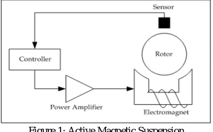
Generation of contact free magnetic field forces by actively controlling the dynamics of an electromagnet is the principle which is actually used most often among the magnetic suspensions. The schematic of the function principle of the active electromagnetic suspension is shown in the figure-1.

Figure 1: Active Magnetic Suspension

The sensor senses the air gap between the rotor and the electromagnet. The voltage signal is given to controller and the current output from the controller is amplified by the power amplifier and feed in to the coil in the electromagnet. This control current controls the rotation of rotor. Initially the rotor rests on the touch down bearing and with the current input the rotor is get lifted from its position and starts rotating. The entire control loop is get controlled by the control current and any change in the required current leads to the unbalance of the rotor and the suddenly fall on the touch down bearing, which prevents the falling of the rotor in the bearings and damage of the system. Touch down bearing provides safe landing of rotor and smooth rundown in the time of failure of suspension electronics or loss of power supply while rotating.

IV. SYSTEMMODELLING

Technology (IJRASET)

©IJRASET 2015: All Rights are Reserved

153

which simplifies the realized bearing stiffness in a physically reasonable range. (b) The bearing force characteristics do not show its dependency on coil current, rotor position and other physical quantities. The linearized force/current and force/displacement relation at the operating point is represented as:

( , ) =− + (1)

The open loop active magnetic bearing system given by (1) is unstable dynamic system which can be stabilized by a suitable controller essentially comes down to finding an appropriate current commanding signal i. The control current is expressed as a function of the rotor displacement x and its time derivative:

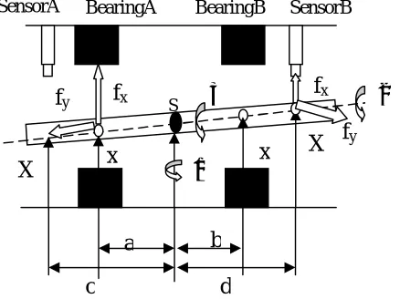
( ) =−( ) ̇ (2)

Rotor dynamics refers to the classical results of vibration theory and gyro mechanics which deals with the natural vibrations, forward and backward whirl, critical speed or nutation and precession. An elastic supported body can undergo natural as well as forced vibrations. The basic structure of the rigid rotor is shown by the figure-2:

Figure 2: Basic rigid rotor structure

The generalized forces Zi depends on the bearing forces f:

= = (3)

where;

=

0 0

1 1 0 0

0 0

0 0 1 1

(4)

The basic equation of motion for a rigid rotor in linear analysis can be represented as:

̈+ ̇+ = 0 (5)

where , G and are termed as mass, gyroscopic and stiffness matrices with = [ , ,− , ] of which and are termed as angular motion and, and are termed as translational motions. In general translational and rotational motions will be coupled.

S

Ω

α

α

β

x

A

x

a

b

X

X

c

d

f

f

f

Technology (IJRASET)

©IJRASET 2015: All Rights are Reserved

154

=

0 0 0

0 0 0

0 0 0

0 0 0

(6)

=

0 0 1 0

0 0 0 0

−1 0 0 0

0 0 0 0

Ω (7)

The equations here characterize the mass and stiffness distribution within a mechanical system. This system is conservative i.e. it does not show any energy dissipation and thus it is limit stable if for the stiffness matrix K>0 holds: in other words if its statically stable. Such a system cannot be destabilized by gyroscopic forces and therefore it will remain stable at any rotor speed.

The usual model for the vibrational motions of a rotor system with no excitations acting on it, and somewhat with respect to the (5) is the homogenous, linear system of equations:

̈+ ( + ) ̇+ ( + ) = 0 (8)

where D is the damping matrix and N is the non-conservative bearing forces

Oneof the nonlinear quantities that affect the performance of the system is gyroscopic effect. The tilt of a rotating shaft relative to the axis of rotation generates gyroscopic disturbances [15]. In the modeling and analysis of rotor-dynamic systems, there are two main phenomena that are attributed to the gyroscopic effects. First, the gyroscopic moments tend to couple the dynamics in the two radial directions of motions. Second, gyroscopic moments cause the critical speeds of the system to drift from their original predictions at zero speed. While including the gyroscopic effects the equation (5) can be changed to equation (9), where represents angular velocity of the rotor. M, G and K are matrices representing mass gyroscopic effect and stiffness.

̈+ ̇+ = 0 (9)

Another nonlinear component which may affect rotor dynamics due critical speed of rotor is whirling. Due to critical speed, the rotor may whirl forward [20]. Considering the whirling motion of rotor, the equation can me modified as

̈+ ̇+ = (10)

The right hand side of the equation determines the harmonic excitation. The response is characterized by frequency response. The

Us component that can only excite the natural frequency which will whirl in the same direction of the rotor spin which is shown below:

= − (10a)

= [ ] (10b)

The equations (10a) and (10b) are considered for forward whirling of rotor; where e is the eccentricity i.e. the deviation of center of mass from geometric centre of rotor and represents the rotation of the horizontal axis of rotor. The equation (10c) is comprises of the Us component which is considered in the case of backward whirling of the rotor.

= 1

0 0

Technology (IJRASET)

©IJRASET 2015: All Rights are Reserved

155

Static and dynamic unbalances are another nonlinear effect which occurs due to eccentricity and inclination of the principle axis

of inertia. When the rotor is rotating with speed the resulting centrifugal force acting on one of the additional masses ∆ and rotating together with rotor is:

= ∆ 0 0 (11a)

For a static unbalance, the centrifugal forces acting up on the two small additional masses can be combined in to a resulting force through centre of mass S. For dynamic unbalance, the centrifugal forces start acting in opposite directions, in other words we can say that there is a couple due to these forces about axis resulting in a torque. The same can be represented mathematically as follows:

= [0, , 0] (11b)

where;

= 2 = 2 ∆ = (11c)

Vibrations are another nonlinear component that affects the stability of suspension of the system. It comprises of tortional [16] and damped and undamped free vibrations [19]. Equation (12) shows the basic equation for tortional vibration and equation (13) and (14) shows the damped and undamped free vibrations.

[ ] ̈ + [ ] ̇ + [ ]{ } = 0 (12)

for which is the diagonal inertial matrix and and are damping matrices and shows the angular displacement vector in radians, ̇ shows the angular velocity in radians/sec and ̈ represents the angular acceleration vector in radians/square seconds.

̈ + + ̇ = 0 (13a)

̈ + + ̇ = 0 (13b)

̈ + = 0 (14a) ̈ + = 0 (14b)

where the geometric center of the disk is located at the point ( , ) along coordinate axis defined about the bearing center line and M, and represents the mass, stiffness and damping matrix of the rotor. The damping component and unbalance eccentricity in the undamped free vibration is considered to be zero [19].

Mostly vibration in the suspension is due to the unbalance which comprises of static and dynamic unbalance [17]. Fedák in [15] discusses on the basic equations for static and dynamic unbalances (shown in equation (15) and (16)).

̈+ ̇+ = cos( ) (15a)

̈+ ̇+ = sin( ) (15b)

Technology (IJRASET)

©IJRASET 2015: All Rights are Reserved

156

̈ ₊ ̇ _{+ = ( ) (16a)} ̈ − ̇ _{+ = ( ) (16b)}

In the above equations (16a) and (16b) represents the torque caused by unbalance. is the transverse moment of inertia and the polar moment of inertia.

In the closed loop systems including the nonlinear effects, k is considered to be feedback vector. The method is based on matrices operations that describe the system model, and for this reason, the inner state of the process can be accessed, not only inputs and outputs. For this, firstly decoupling of MIMO system is done to find an approximate model consisting of two or more SISO systems [3]. A continuous, linear, constant-coefficient system of differential equations can always be expressed as a set of first-order matrix differential equations:

x(k + 1) =∅ x(k) +Γ u(k) (17a)

y(k) = Hx(k) (17b)

with = [1 0]. In equation (11); x is the inner states vector, u is the control input vector and y represents the outputs vector and ∅

represents the rotational angle between the rotor and the horizontal axis. The most attractive feature about state space controller method is that the procedure has two steps which includes firstly assuming that all the states are known and estimator is designed, in order to estimate the inner state vector. Thus the control law consists of combination of control law and estimator, with control law calculations based on estimated state. The state vector is considered to be in two parts: represent part directly measured (rotor position) or calculated respectively (rotor movement speed), and is the remaining portion to be estimated (i.e. gravitation and disturbance force).

( + 1)

( + 1) = +

Γ

Γ ( )

(18a)

( ) = ( )_{( )} (18b)

V. SIMULATIONRESULTS

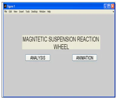
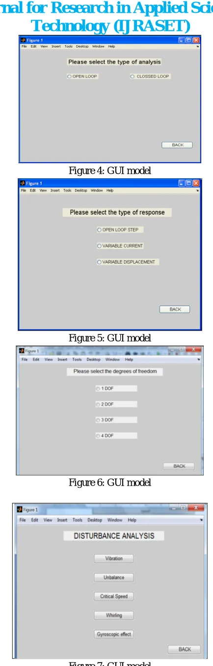
The developed GUI model in figure-3 to 7 is characterized by using linear and non-linear analysis for open loop and closed loop conditions.

Technology (IJRASET)

©IJRASET 2015: All Rights are Reserved

157

Figure 4: GUI model

Figure 5: GUI model

Figure 6: GUI model

Technology (IJRASET)

©IJRASET 2015: All Rights are Reserved

158

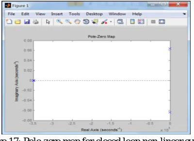
The model is tested using the following parameters and its response is also listed in the different cases given below:

Parameters Values Rotating speed of the rotor 7000 rpm Distance between rotor and

bearing A 20.3 mm Distance between rotor and

bearing B 20.3 mm Distance between rotor and

sensor A 20.3 mm Distance between rotor and

sensor B 20.3 mm Inertia along X-axis 200 NS2/m Inertia along Y-axis 200 NS2/m Inertia along Z-axis 200 NS2/m Rotor mass 4 kg Radial stiffness of rotor 200 Nm Axial stiffness of rotor 200 Nm

Table 1: System parameters used for testing

Case-1: Linearized force/current & force/displacement equation

Analyzing the basic force equation for the system, the system response obtained for both varying current and varying displacement is shown in figure-8 and figure-9.

Figure 8: Variable current plot

Technology (IJRASET)

©IJRASET 2015: All Rights are Reserved

159

Case-2: Analysis for linear open loop system

The step response analyses with the open loop configuration have a highly unstable behavior as shown in the figure-10.

Case-3: Analysis for linear closed loop system

Modeling the above discussed force equation; the obtained the closed loop linear response figure-11 shows the system is stable while considering the feedback loop.

Figure 10: Open loop step response of a linear system

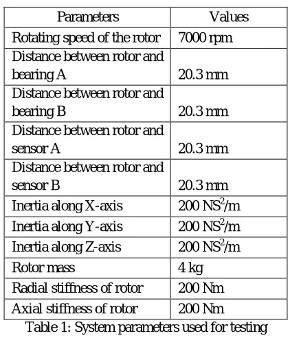
In the linear analysis the system is stable as no nonlinear effects are being considered. But considering the practical study, so many nonlinearities may affect the system which leads to the unbalance of rotor and finally may cause the damage of entire system. Hence the nonlinear analysis became important for the actual study of the system. The effect includes gyroscopic, static and dynamic unbalance, vibration, effects due to critical speed etc. For e.g. critical speed leads to whirling of rotor and due to unbalance, the system may vibrate.

Figure 11: Pole-zero map for linear closed loop system

Case-4: Analysis for the nonlinear effects on open loop rigid rotor

Figure-12 and 13 shows the step response and pole-zero plot for the static unbalance while adding additional mass. Static unbalance is adjusted by adding balancing masses in same plane or by removing additional mass from same plane and the removal of dynamic unbalance is studied by adding balancing masses in same plane or by removing adding masses from different planes.

Technology (IJRASET)

©IJRASET 2015: All Rights are Reserved

160

Figure 13: Pole-zero plot for adding balancing mass in static unbalance analysis

From figure-13, it has been analyzed that the system is marginally stable based on the input parameters.

Similarly the analysis has been done for removing masses study for static unbalance and adding and removing additional masses for dynamic unbalance have been done. While doing increased speed analysis, due to critical speed the rotor may whirl forward. Whirling is of both forward and backward directions. The figure-14 shows the pole-zero plot for the forward whirling of rotor due to critical speed.

Figure 14: Pole-zero plot for Critical speed analysis Similarly stability analyses for both the whirling effects have been done.

Technology (IJRASET)

©IJRASET 2015: All Rights are Reserved

161

Vibration is of great concern for large, flexible spacecraft; that have extremely precise positional and vibratory tolerance requirements, and therefore there is a need for vibration reduction. Vibration results in the unbalance of the rotor. Stability analyses have been done for there types of vibrations (tortional, damped and undamped vibration) have been done. The above discussed constitutes the open loop nonlinear analysis of the system. As already discussed the open loop systems are highly unstable systems which makes the study of nonlinear systems to be important.

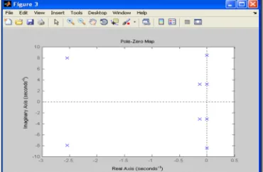
Case-5: Analysis of closed loop system (control loop included)

Analysis has been done by closing the current control loop. A decentralized PD controller has been introduced for the control of the system which is shown in equation (18). Based on the above discussed parameters, the system is found to be marginally stable.

Figure 16: Step response analysis for closed loop non-linear system

Figure 17: Pole-zero map for closed loop non-linear system

In the state space analysis of the radio servo loop (transfer function diagram for one degree of freedom) i.e. in one degree of freedom the result obtained which is shown in figure-16. The radio servo loop is a feedback loop in one degree of freedom which will be in radial direction. From the study it is understood that the system is stable.

Technology (IJRASET)

©IJRASET 2015: All Rights are Reserved

162

Figure 19: Step response of controller in radio servo loop

In the analysis of the controller alone; the step and the frequency response analysis have been done which is shown in figure-17 and 18.

Figure 20: Frequency response analysis of controller in radio servo loop

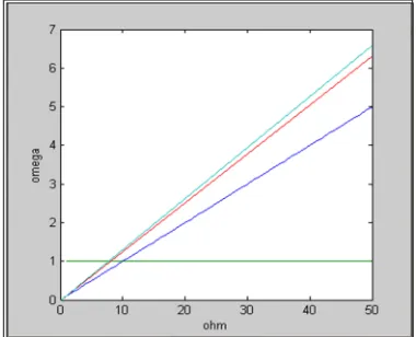
Figure-19 represents the graphical response of eigen value dependence on the rotor speed for an elastically supported rigid rotor. Also the analysis has been done for different values of speed which is shown in figure-20.

Technology (IJRASET)

©IJRASET 2015: All Rights are Reserved

163

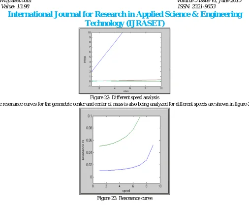
Figure 22: Different speed analysis

The resonance curves for the geometric center and center of mass is also being analyzed for different speeds are shown in figure-21.

Figure 23: Resonance curve

VI. CONCLUSION

This paper describes the development and analysis of a Graphical User Interface (GUI) model using Matlab for Magnetic Suspension Reaction Wheel (MSRW). The GUI has been provided with the features of configuring the system in open loop and closed loop mode, flexibility regarding the selection of the various degrees of freedom as well as the inclusion of various disturbance analysis such as unbalance, vibration, gyroscopic effects etc. The developed model has been tested for the parameters listed in the paper and the simulated results are also presented.

As a scope of improvement the work can be extended by interfacing the developed GUI with the actual system and validation of the same.

REFERENCES

[1] U. J. Bichler; A low noise magnetic Bearing Wheel for space application; Second International Symposium on Magenetic Bearing, July 12-14, 1990, Tokyo, Japan.

[2]Wei-Yong Zhou, GuglielmoS.Aglietti and ZheZhang, Modeling and testing of a soft suspension design for a reaction/ momentum wheel assembly; College of Aerospace and material engineering, National university of defence, People’s republic of China.

[3] Chip Rinaldi Sabirin, Andreas Binder, Dumitru Daniel Popa and Aurelian Craciunescu; Modeling and digital control of an Active Magnetic Bearing system; Technische Universität Darmstadt, Institut fur Elektrische Energiewandlung, Landgraf-Georg-Str. 4, Darmstadt, and “Politehnica” University of Bucharest, Electrical Engineering Department 313 Splaiul Independentei, Bucharest

[4] L.Trumper, Linearizing Control of Magnetic Suspension Systems; IEEE transactions on control systems technology, vol. 5

[5] Ishtiaq Ahmad and Muhammad Akram Javaid, Nonlinear Model & Controller Design for Magnetic Levitation System; Department of Civil Engineering and Department of Basic Sciences University of Engineering & Technology, Pakistan

[6] John Watkins and Ken Blumen stock, Control of integrated radial and axial bearing; Systems Engineering Department, US. Naval Academy and Electromechanical Systems Branch; NASA

Technology (IJRASET)

©IJRASET 2015: All Rights are Reserved

164

China

[8] M. L. Dertouzos and J. K. Robergen, High capacity reaction wheel attitude control; Members IEEE

[9] Mulukuta S. Sarma, Akira Yamamura Nonlinear Analysis of Magnetic Bearings for Space Technology; IEEE transactions on aerospace and electronic systems, 2012

[10] Radoslav N. Tomović, Mathematical model of dynamic behavior of rigid rotor inside the rolling element bearing; 13th International Research/Expert Conference ”Trends in the Development of Machinery and Associated Technology” TMT 2009, Hammamet, Tunisia

[11] S. Myburgh, G. van Schoor, E.O. Ranft, A Non-linear Simulation Model of an Active Magnetic Bearings Supported Rotor System; International Conference on Electrical Machines - ICEM 2010, Rome

[12] Tingshu Hu ,Zongli Lin, Wei Jiang and Paul E Allaire, Constrained control design for magnetic bearing systems; Department of electrical and computer engineering

[13] W. de Boer, Active Magnetic Bearings: Modelling and control of a five degrees of freedom rotor Master of Science Thesis; December1998 Department of electrical engineering of the Eindhoven university of technology; Measurement and Control Group

[14] D. L. Trumper, J. Sanders, T. Nguyen, and M. Queen, “Experimental results in nonlinear compensation of a one-degree-of-freedom magnetic suspension,” in Proc. NASA Int. Symp. Magn. Suspension Techonol., NASA Langley Research Center

[15] Viliam Fedák, Pavel Záskalický and Zoltán Gelvanič ; Analysis of Balancing of Unbalanced Rotors and Long Shafts using GUI MATLAB; MATLAB Applications for the Practical Engineer; Intech

[16] J.C. Wachel and Fred R. Szenasi; Analysis of tortional vibrations in rotating machinery; President and Senior project engineer; Engineering dynamics incorporated; San Antonio; Texas

[17] BRÜEL and KJAER Static and Dynamic Balancing of Rigid Rotors.; Application notes. Germany: Naerum Offset; 1989

[18] Jianrong CAO, Quanshi CHEN; Decoupling Control for a 5-Dof Rotor Supported by Active Magnetic Bearings; State Key Laboratory of Autoinotive Safety and Energy Tsingliua University Beijing, P.R. China I00084; E-mail: caojr~tsinghua.edu.cn