Model based analysis of oligonucleotide arrays: model validation, design issues and standard error application

comment

reviews

reports

deposited research

interactions

information

refereed research

Research

Model-based analysis of oligonucleotide arrays: model validation,

design issues and standard error application

Cheng Li* and Wing Hung Wong*

†

Addresses: *Department of Biostatistics, Harvard School of Public Health, 655 Huntington Avenue, Boston, MA 02115, USA. †_{Department of}

Statistics, Harvard University, One Oxford Street, Boston, MA 02138, USA.

Correspondence: Wing Hung Wong. E-mail: [email protected]

Abstract

Background: A model-based analysis of oligonucleotide expression arrays we developed previously uses a probe-sensitivity index to capture the response characteristic of a specific probe pair and calculates model-based expression indexes (MBEI). MBEI has standard error attached to it as a measure of accuracy. Here we investigate the stability of the probe-sensitivity index across different tissue types, the reproducibility of results in replicate experiments, and the use of MBEI in perfect match (PM)-only arrays.

Results: Probe-sensitivity indexes are stable across tissue types. The target gene’s presence in many arrays of an array set allows the probe-sensitivity index to be estimated accurately. We extended the model to obtain expression values for PM-only arrays, and found that the 20-probe PM-only model is comparable to the 10-probe PM/MM difference model, in terms of the expression correlations with the original 20-probe PM/MM difference model. MBEI method is able to extend the reliable detection limit of expression to a lower mRNA concentration. The standard errors of MBEI can be used to construct confidence intervals of fold changes, and the lower confidence bound of fold change is a better ranking statistic for filtering genes. We can assign reliability indexes for genes in a specific cluster of interest in hierarchical clustering by resampling clustering trees. A software dChip implementing many of these analysis methods is made available.

Conclusions:The model-based approach reduces the variability of low expression estimates, and provides a natural method of calculating expression values for PM-only arrays. The standard errors attached to expression values can be used to assess the reliability of downstream analysis.

Published: 3 August 2001

GenomeBiology2001, 2(8):research0032.1–0032.11

The electronic version of this article is the complete one and can be found online at http://genomebiology.com/2001/2/8/research/0032 © 2001 Li and Wong, licensee BioMed Central Ltd

(Print ISSN 1465-6906; Online ISSN 1465-6914)

Received: 15 February 2001 Revised: 7 May 2001 Accepted: 13 June 2001

Background

The statistical model proposed in [1] for one probe set in multiple oligonucleotide arrays has the form

yij= PMij– MMij= qifj+ eij,

兺

2_{= J, e}

ij~ N冸0, s2冹 (1)

It states that the perfect match (PM)/mismatch (MM)

differ-ence in array i, probe jof this probe set is the product of

model-based expression index (MBEI) in array i (qi) and

probe-sensitivity index of probe j (fj) plus random error.

Here Jis the number of probe pairs in the probe set. Fitting

the model, we can identify cross-hybridizing probes (fjwith

large standard error (SE), which are excluded during itera-tive fitting) and arrays with image contamination at this

probe set (qiwith large SE), as well as single outliers (image

estimated expression index qi is a weighted average of

PM/MM differences:

qi ~

= 冸

兺

j yijfj冹兾J,

with larger weights given to probes with larger f. The image

of outliers (array and single outliers) identified through model-fitting can be used to assess the quality of an experi-ment and to identify unexpected problems such as a mis-aligned corner of a DAT file [1].

We have investigated several important properties of the model, including the reliability and stability of the fitted

parameters MBEI (q) and probe sensitivity indexes (f), the

performance of MBEI compared to the commonly used average difference (AD), and how the availability of SE facili-tates downstream comparative and clustering analysis.

Results and discussion

Probe-sensitivity indexes are stable across tissue types In practice, in an array experiment, a researcher hybridizes tissue or cell line samples, corresponding to different treat-ments or conditions, to a batch of arrays. Ideally, the

probe-sensitivity index (f) should be independent of the tissue

type. This condition, however, may not hold for those probes that have cross-hybridization affinity to non-target genes. Nevertheless, assuming that a non-target gene cross-hybridizes only to a few probes of a probe set, and its expression levels across arrays do not correlate with the target gene, the iterative probe-excluding procedure in [1] may be able to exclude cross-hybridizing probes, regardless of the tissue type hybridized. In addition, the relative probe-sensitivity indexes of the good probes called by the model are likely to be similar across sets of arrays hybridizing to different tissue samples.

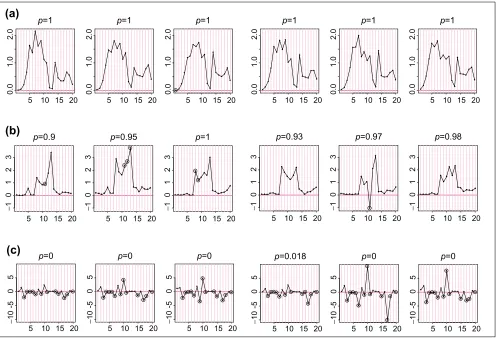
The stability of the probe-sensitivity index is studied using 226 HU6800 arrays. We apply the model (equation 1) independently to six sets of HU6800 arrays (21 leukemia, lymphoma and mantle cell samples, 20 prostate cancer cell lines, 17 brain tumor samples, 55 cancer cell lines, 58 brain samples, and 55 lung tumor samples). Figure 1a shows the

fvalues fitted for probe set 6457 (used in Figure 1 and 2 of

[1]) in the six array sets. The f patterns resemble each

other greatly, showing that the probe-sensitivity index is an inherent property of these non-cross-hybridizing probes and can be consistently identified from different sets of

arrays. Figure 1b shows the f patterns for another probe

set. It is noteworthy that the probe 11 in array set 5 is likely to be cross-hybridizing, making its relative strength (here MM is consistently larger than PM and this leads to a

nega-tive f) dissimilar to the probe 11 in other array sets. The

model identifies this probe as a ‘probe-outlier’ only for

array set 5 and excludes it when calculating MBEI (q) for

array set 5.

In Figure 1a,b the target gene is present in most samples of all array sets. For a probe set whose target gene is mostly absent throughout samples (Figure 1c), many probes are identified as probe-outliers because of their negative indexes. Here, we cannot obtain correct probe-sensitivity indexes because of the absence of the target gene. Neverthe-less, the PM-MM values for these probes are random fluctu-ations around zero, leading to a correct expression index close to zero. If the target gene becomes available for a future array set, the correct probe-sensitivity indexes will be recovered and these probes will be used for expression calculation.

Occasionally, a responsive probe set may give rise to very

different festimates in two array sets. In Figure 1b, probes 8

and 13 have different relative responses in array set 1 and 4, leading to different probe-response patterns. This might be due to the possibility that the probes in this probe set are dif-ferentially cross-hybridized in different array sets, or that the same probe in different batches of arrays may systemati-cally behave differently. Identification and flagging such probe sets is desirable and essential if we want to compare arrays hybridized to different tissue samples.

Figure 2 shows the boxplots of average pairwise correlations

of f values between two array sets, stratified by average

lower presence proportion in the two sets. In general, when a

gene is present in many samples of two array sets, the f

pat-terns estimated from the two sets are very similar. The target gene’s presence in many arrays of an array set allows the probe-sensitivity index to be estimated accurately.

Model-based analysis for PM-only arrays

From Figure 1 of [1], one can see that some MM probes may respond poorly to the changes in the expression level of the target gene. This phenomenon raised questions on the effi-ciency of using MM probes, and led some investigators to design custom arrays that use PM probes exclusively (R. Abagyan and Yingyao Zhou, personal communication; B.R. Conklin, personal communication), and others to calcu-late fold changes using only PM probes (F. Naef, personal communication). This design greatly increases the number of genes that can be studied on one array. To investigate the relative performance of PM/MM versus PM-only designs, we exploited the model to estimate gene expression levels using only PM probes, and compared it to the MBEI using both PM and MM probes.

The full intensity model (equation 1 of [1]) specifies the

rela-tionship of PM probe responses and expression level q:

PMij= nj+ qifj¢ (2)

where njis the baseline response of probe pair jdue to

non-specific hybridization, and f¢

jis the sensitivity of PM probe

of the probe pairj. The parameter estimates can be obtained

comment reviews reports deposited research interactions information refereed research

known. The same outlier exclusion procedure in [1] is applied. The MM probe responses have a similar form as equation 2 except for different probe-sensitivity indexes. We fit a PM-only and an MM-only model to obtain expression values of all 20-probe probe sets using array set 1. For com-parison, we also used half of the probe pairs (by alternatively picking one out of every two probes) in a 20-probe probe set to fit to the difference model (equation 1). For each probe set, these three sets of expression values were compared with the expression values of the original difference model

using 20 probes, in terms of correlation of qs obtained by

two methods across the 21 arrays. We assumed the 20-probe difference model provides the most accurate expression esti-mates. If, for a probe set, a simplified model (PM-only, MM-only or 10-probe difference model) performs

reason-ably well, we expect its q estimates to correlate with that

from the 20-probe difference model.

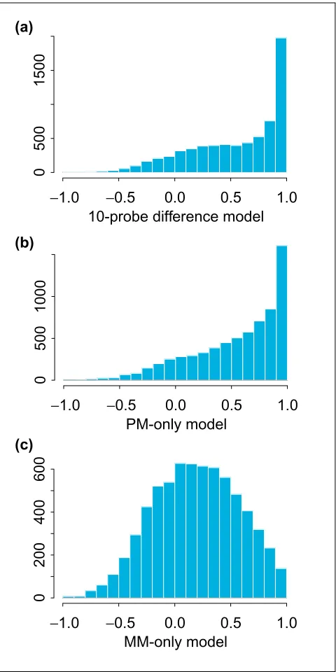
Figure 3 shows the histogram and Figure 4 the boxplot of

correlations of qs estimated from the 20-probe difference

model and qs estimated from the 10-probe difference model

(a), the 20-probe PM-only model (b) and the 20-probe MM-only model (c). For probe sets with high presence pro-portion, both the 10-probe difference model and the PM-only model correlate well with the 20-probe difference model. The MM-only model yields noticeably lower correlations, however. We note that this comparison is intrinsically biased in favor of the 10-probe difference model because the ‘truth’ is constructed from PM-MM differences.

This comparison corroborates the basic notion of the tech-nology: the PM probes hybridize more strongly to the target signals than MM probes and contain most of the informa-tion. We stress that, whereas the above analysis illustrates the applicability of model-based analysis to PM-only arrays, the assessment presented here is only tentative because of the limited information provided by the HU6800 arrays on the comparisons. Definitive comparisons of the efficiency of the designs must await the availability of data from PM-only arrays.

Figure 1

fvalues for probe sets. fvalues estimated for probe sets (a)6457, (b)1248, and (c) 6571 in six array sets (shown in panels 1-6 from left to right for each probe set). fvalues (constrained to have sum square equal to number of probes used in each array set) are on the y-axis, and probe pairs are labeled 1 to 20 on the x-axis. The title of each panel (for example, p = 0) indicates the proportion of arrays ‘present’ for the target gene in the array set. Large circles represent identified probe-outliers by negativity or large SE of f.

5 10 15 20

0.0

1

.0

2.0

p=1

5 10 15 20

0.0

1

.0

2.0

p=1

5 10 15 20

0.0

1

.0

2.0

p=1

5 10 15 20

0.0

1

.0

2.0

p=1

5 10 15 20

0.0

1

.0

2.0

p=1

5 10 15 20

0.0 1 .0 2.0 p=1

(a)

5 10 15 20

− 10 1 2 3 p=0.9

5 10 15 20

− 10 1 2 3 p=0.95

5 10 15 20

− 10 1 2 3 p=1

5 10 15 20

−

1

0

123

p=0.93

5 10 15 20

−

1

0

123

p=0.97

5 10 15 20

− 1 0 123 p=0.98

(b)

5 10 15 20

− 10 -5 0 5 p=0.018

5 10 15 20

− 10 -5 0 5 p=0

5 10 15 20

− 10 -5 0 5 p=0

5 10 15 20

− 10 -5 0 5 p=0

5 10 15 20

− 10 -5 0 5 p=0

5 10 15 20

MBEI reduces variability for low expression estimates The array set 5 has 29 pairs of arrays [2]. Each pair consists of two arrays hybridizing to samples replicated at total mRNA level (the total mRNA sample is split and then amplified and labeled separately, and hybridized to two different arrays). The differences between the expression values of the two replicate arrays in a pair are due to the variation introduced in experimental steps after the split, the array manufacturing difference and analytical methods such as normalization and expression calculation. This difference provides a lower bound of biological variation that can be detected between two independently amplified samples, and serves as a good statistic for comparing different analytical methods.

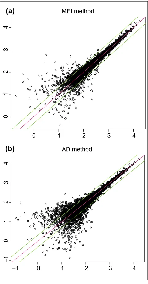
The agreement of MBEI between two replicate arrays is shown in Figure 5a. For comparison, we also used the method in [3] to calculate ADs for all probe sets and plot them in Figure 5b (AD is based on normalized probe values, see Methods and materials section for the normalization method. Also note that GeneChip software excludes probes whose PM/MM difference is outside three standard deviations

(SDs) of all probe differences in either of the two arrays in the comparison; here, as we are comparing multiple arrays at the same time, when calculating ADs a probe is excluded if its dif-ference is an outlier in the above sense in any of the arrays, until a minimum of five probes is reached, where all five probes will be used). Both the MBEI and the AD method Figure 2

Boxplots of average pairwise correlations of fs between two array sets. They are stratified by average lower presence proportion in two array sets (the presence proportion of a probe set is the proportion of arrays in an array set where the target gene is called ‘present’ by

GeneChip’s algorithm). The average is taken over C(6, 2) = 15 pairwise comparison of two array sets for each probe set, and the correlation is calculated using probes that are not identified as an outlier in both array sets. The range of the average lower presence proportion for the six boxplots are: (0, 0.17), (0.17, 0.34), (0.34, 0.51), (0.51, 0.68), (0.68, 0.85), (0.85, 1). The title of each boxplot is the number of probe sets classified into this boxplot. Eleven probe sets with too few non-outlier probes to calculate fcorrelations for all 15 comparisons are not included in the boxplots. The average lower presence proportion and average pairwise correlation for probe sets in Figure 1 are (a) 1, 0.95; (b), 0.93, 0.94; and (c) 0, 0.86.

−

0.2

0.0

0.2

0.4

0.6

0.8

1.0

4150

−

0.2

0.0

0.2

0.4

0.6

0.8

1.0

920

−

0.2

0.0

0.2

0.4

0.6

0.8

1.0

575

−

0.2

0.0

0.2

0.4

0.6

0.8

1.0

503

−

0.2

0.0

0.2

0.4

0.6

0.8

1.0

422

−

0.2

0.0

0.2

0.4

0.6

0.8

1.0

548

Figure 3

Histogram of correlations between model-based expression values estimated using the 20-probe difference model and those estimated using different models. (a)10-probe difference model; (b)20-probe PM-only model; (c)20-probe MM-only model. All comparisons are across the 21 arrays in array set 1.

−

1.0

−

0.5

0.0

0.5

1.0

0

500

1500

10-probe difference model

−

1.0

−

0.5

0.0

0.5

1.0

0

500

1000

PM-only model

−

1.0

−

0.5

0.0

0.5

1.0

0

200

400

600

MM-only model

(a)

(b)

yielded some expression values differing by more than a factor of two, especially for genes at low expression level. This might be explained by the relatively larger amplification vari-ation for weakly expressed genes, given a constant success rate of amplifying a sequence by a certain fold.

Researchers often use ‘log ratio’ between expression values of a gene in two arrays as the criterion for identifying differ-entially expressed genes. Between duplicate arrays, we expect these log ratios of expression values based on a good expression index (AD or MBEI) to be close to zero. Thus for every probe set we calculated its average absolute log (base 10) ratio of 29 pairs of duplicates as a statistic to compare the variation in expression levels between duplicates using

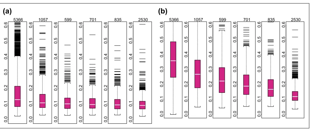
the AD or the MBEI method. Figure 6 presents the results of the comparison. The average absolute log ratio distribution of the MBEI method is significantly lower than that of the AD method when expression level is low (and thus probe sets have a low proportion of detections of the target gene across arrays). As expression level becomes higher (when the target gene of a probe set is detected in more arrays), the AD method shows a rapid improvement in performance, approaching the level of the MBEI method. The same box-plots (Figure 7) for another set of 60 human U95A arrays consisting of 30 replicate pairs conveys similar information. These results suggest that the MBEI method is able to extend the reliable detection limit of expression to a lower mRNA concentration. comment reviews reports deposited research interactions information refereed research Figure 4

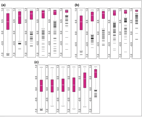
Boxplot of correlations between qvalues estimated using the 20-probe difference model and qs estimated using different models, stratified by presence proportion. (a) 10-probe difference model; (b)20-probe PM-only model; and (c) 20-probe MM-only model. The number of presence calls for a probe set in the 21 arrays and the subpopulation size for the six boxplots are: 0–3, 4,385; 4-7, 693; 8-11, 413; 12-15, 488; 16-19, 497; and 20-21, 323. Only 6,799 probe sets that have 20 probes are used.

Confidence interval for fold change

After obtaining expression indexes using AD or MBEI, fold changes can be calculated between two arrays for every gene and used to identify differentially expressed genes. Usually, low or negative expressions are truncated to a small number before calculating fold changes, and GeneChip also cautions against using fold changes when the baseline expression is absent.

The availability of SEs for the model-based expression indexes allows us to obtain confidence intervals for fold changes. Suppose

q

^_{1~ N冸q1, d1}2_{冹, q}^

2~ N冸q2, d22冹

where q1and q2are the real expression levels in the sample,

and^q1and ^q2are the model-based estimates of expression

levels. We substitute the model-based SEs for d1 and d2.

Letting r= q1/q2be the real fold change, then inference on r

can be based on the quantity

冸q^1– rq^2冹2 Q = ———————

d12+ d22r2

It can be shown that Q has a c2_{distribution with 1 degree of}

freedom irrespective of the values of q1and q2[4]. Thus Q is

a pivotal quantity involving r. We can use Q to construct

fixed-level tests and to invert them to obtain confidence intervals (CI) for fold changes [5].

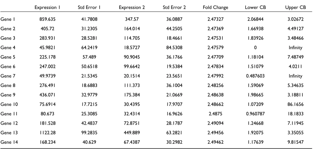
Table 1 presents the estimated expression indexes (with SEs) in two arrays and the 90% confidence intervals of the fold changes for 14 genes. Although all genes have similar esti-mated fold changes, the confidence intervals are very differ-ent. For example, gene 1 has fold change 2.47 and a tight confidence interval (2.06, 3.02). In contrast, gene 11 has a similar fold change of 2.48 but a much wider confidence interval (0.96, 18.18). Thus the fold change around 2.5 for gene 11 is not as trustworthy as that for gene 1. Further examination reveals that this is due to the large SEs relative to the expression indexes for gene 11. This agrees with the intuition that when one or both expression levels are close to zero for one gene, the fold change cannot be estimated with much accuracy. In addition, when image contamination results in unreliable expression values with large SEs, the fold changes calculated using these expression value are attached with wide CIs. In this manner, the measurement accuracy of expression values propagates to the estimation of fold changes.

In practice, we find it useful to sort genes by the lower confi-dence bound (‘Lower CB’ in Table 1), which is a conservative estimate of the fold change. When an expression index is negative (as a result of taking PM/MM differences), we do not calculate the confidence intervals. In such a case, it is more helpful to filter genes by presence calls.

Standard errors help to assess clustering results Cluster analysis is a popular method for analyzing the data of a series of microarrays [6,7]. If two genes are co-regulated at the transcription level, their expression values across samples are likely to be correlated. Clustering algorithms use these correlations (or monotone transformation of correla-tions) to cluster co-regulated genes together. The correlation based on the estimated expression levels may, however, be Figure 5

Log (base 10) expression indexes of a pair of replicate arrays (array 1 and 2 of array set 5) for different statistical

methods. (a) MBEI method; (b)AD method. Only 6,695 (a) and 4,696 (b) probe sets with positive values in both arrays are used. The center line is y= x, and the flanking lines indicate the difference of a factor of two.

MEI method

(a)

0 1 2 3 4

01

2

3

4

−1 0 1 2 3 4

−

10

1

2

3

4

different from that based on the real but unobserved expres-sion levels. Also, the commonly used hierarchical clustering algorithm is an irreversible process: once two genes or nodes are merged, they will stay together, even if later on there is good reason to adjust previous clustering. Thus there is a need to assess the reliability of clusters.

A global way of using SE in hierarchical clustering is to resample or bootstrap [8] the whole ‘gene by sample’ data matrix and redo the clustering, then investigate the overall properties emerging from this repertoire of clustering trees.

In Bittner et al. [9], the data matrix coming from cDNA

microarray experiments is resampled using the estimated

comment reviews reports deposited research interactions information refereed research Figure 6

Boxplots of average absolute log (base 10) ratios between replicate arrays stratified by presence proportion for different statistical methods. (a)MBEI method; (b)AD method. The number of presence calls for a probe set in the 58 arrays for the six boxplots are: 0-9, 10-19, 20-29, 30-39, 40-49, 50-58. The title of each boxplot is the number of probe sets used for the boxplot. The average is taken over 29 replicate pairs. Log ratios are not calculated for negative expression values or expression values identified as ‘array-outliers’ by the MBEI method in either array of a replicate pair, and are not used to calculate the average. 744 probe sets are not included as their average absolute log ratios cannot be calculated for all the 29 pairs using either method.

0.0 0.1 0.2 0.3 0.4 0.5 0.6 2693 0.0 0.1 0.2 0.3 0.4 0.5 0.6 677 0.0 0.1 0.2 0.3 0.4 0.5 0.6 485 0.0 0.1 0.2 0.3 0.4 0.5 0.6 466 0.0 0.1 0.2 0.3 0.4 0.5 0.6 438 0.0 0.1 0.2 0.3 0.4 0.5 0.6 1626 0.0 0.1 0.2 0.3 0.4 0.5 0.6 2693 0.0 0.1 0.2 0.3 0.4 0.5 0.6 677 0.0 0.1 0.2 0.3 0.4 0.5 0.6 485 0.0 0.1 0.2 0.3 0.4 0.5 0.6 466 0.0 0.1 0.2 0.3 0.4 0.5 0.6 438 0.0 0.1 0.2 0.3 0.4 0.5 0.6 1626

(a)

(b)

Similar plots as in Figure 6 for another set of 30 pairs of duplicated human U95A arrays. (a)MBEI method; (b) AD

method.The number of presence calls for a probe set in the 60 arrays for the six boxplots are: 0-9, 10-19, 20-29, 30-39, 40-49, 50-60. The title of each boxplot is the number of probe sets used for the boxplot.

variation derived from the median SD of log ratios for a gene across samples. As we now have SEs for all data points, we can resample each expression value from a normal distribu-tion with mean equal to the estimated expression value and SD equal to the attached SE.

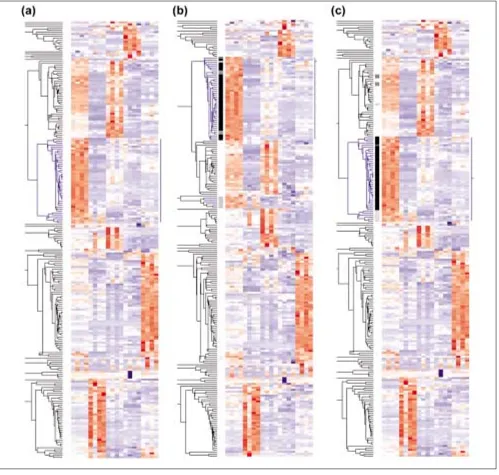
Figure 8a shows a hierarchical clustering tree of 225 selected genes with presence proportion > 0.5 and coefficient of vari-ation (SD/mean) > 0.7 across the 20 samples in array set 2. In trying to interpret this tree, we may be interested in the gene cluster colored in blue and the reliability of the gene members belonging to this cluster. The whole data matrix is resampled, and the clustering is performed again (Figure 8b). We notice that some blue genes (genes in the original cluster are colored blue) are clustered with other non-blue genes, and some non-blue genes are mixed into the main body of the blue genes. After each resampling, we iden-tify a cluster that contains more than 80% of all the blue genes, but as few non-blue genes as possible (measured as a percentage of all genes in this cluster). This cluster is consid-ered to be the cluster that corresponds to the original one in Figure 8a. In Figure 8b the root node of the ‘corresponding cluster’ is marked with small horizontal line intersecting the vertical line (representing the range of the cluster) on the right of the clustering picture. Then, for each of all the 225 genes, if it belongs to this ‘corresponding cluster’, we increase its ‘in-cluster’ count by 1. After resampling 30 times, the in-cluster counts are indicated in gray-scale on the left side of the original clustering (Figure 8c), with black rep-resenting 30 and white reprep-resenting zero. A high ‘in-cluster’

count indicates a gene ‘remains’ in the original cluster in most of the resampled clustering trees.

We can see from Figure 8c that most genes in the original cluster are reliable members, whereas a few genes at the bottom of the cluster are not (in fact they are merged into the original cluster last). Interestingly, some genes originally not in the original cluster group with the ‘corresponding clusters’ during resampling many times and have gray ‘in-cluster’ marks. These genes may be related to the original cluster in some way. In summary, this method can help us to distinguish reliable and unreliable gene members of a cluster, as well as draw our attention to related genes origi-nally clustered somewhere else because of the accidental nature of hierarchical clustering.

Methods and materials

We have developed a software package DNA-Chip Analyzer (dChip [10]) to perform invariant-set normalization (see below), calculation of MBEI [1], computation of confidence intervals of fold changes, and hierarchical clustering with resampling.

Our experience is that more than 10 arrays are appropriate for model training, outlier detection and MBEI calculation. Researchers with fewer than 10 arrays may seek arrays of the same chip type and hybridizing to similar tissue samples, and combine them in a single dChip analysis session. We are

Table 1

Using expression levels and associated SEs to determine confidence intervals of fold changes

Expression 1 Std Error 1 Expression 2 Std Error 2 Fold Change Lower CB Upper CB

Gene 1 859.635 41.7808 347.57 36.0887 2.47327 2.06844 3.02672

Gene 2 405.72 31.2305 164.014 44.2505 2.47369 1.66938 4.49127

Gene 3 283.931 28.5281 114.705 18.4661 2.47531 1.83926 3.48466

Gene 4 45.9821 64.2419 18.5727 84.5308 2.47579 0 Infinity

Gene 5 225.178 57.489 90.9045 36.1766 2.47709 1.18104 7.48749

Gene 6 247.002 50.6518 99.6642 19.5384 2.47834 1.51079 4.0211

Gene 7 49.9739 21.5345 20.1514 23.5651 2.47992 0.487603 Infinity

Gene 8 276.491 18.6883 111.373 36.1004 2.48256 1.59069 5.34635

Gene 9 436.071 32.9779 175.384 21.0669 2.48638 1.98665 3.18811

Gene 10 75.6914 17.7215 30.4395 17.9707 2.48662 1.07209 86.1656

Gene 11 80.673 25.3085 32.4314 16.9626 2.4875 0.960787 18.1833

Gene 12 181.528 42.4837 72.8751 28.1787 2.49094 1.24668 7.11945

Gene 13 1122.28 99.2835 449.889 63.2821 2.49456 1.92075 3.35055

exploring model-based meta-analysis of many arrays of the same chip type but hybridizing to a heterogeneous set of tissues samples, and will present such analysis in future work.

Normalization of arrays based on an ‘invariant set’ As array images usually have different overall image brightness (Figure 9a), especially when they are generated at different

times and places, proper normalization is required before com-paring the expression levels of genes between arrays. Model-based expression computation requires normalized probe-level data (from Affymetrix’s DAT or CEL files). For a group of arrays, we normalize all arrays (except the baseline array) to a common baseline array having the median overall brightness (as measured by the median CEL intensity in an array).

comment

reviews

reports

deposited research

interactions

information

refereed research

Figure 8

A normalization relation can be understood as a curve in the scatterplot of two arrays with the baseline array drawn on

the y-axis and the array to be normalized on the x-axis. A

straight line running through the origin is a multiplicative normalization method (GeneChip’s scaling method), and a smoothing spline through the scatterplot can also be used (Figure 9a, also see [11]).

We should base the normalization only on probe values that belong to non-differentially expressed genes, but generally we do not know which genes are non-differentially expressed (control or housekeeping genes may also be variable across arrays). Nevertheless, we expect that a probe of a non-differ-entially expressed gene in two arrays to have similar intensity ranks (ranks are calculated in two arrays separately). We use an iterative procedure to identify a set of probes (called the invariant set), which presumably consists of points from non-differentially expressed genes (Figure 9b). Specifically, we

start with points of all PM probes (about 140,000 for HU6800 array). If a point’s proportion rank difference (PRD,

absolute rank difference in two arrays divided by n =

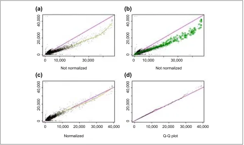
140,000) is small enough, it is kept for the new set. Here the threshold of being small is PRD < 0.003 when a points’s average intensity ranks in the two arrays is small and PRD <0.007 when it is large, accounting for fewer points at high-intensity range; and the threshold is interpolated in between. We chose these parameters empirically to make the selected points in the invariant set thin enough to naturally determine a normalization relation. In this way we may obtain a new set of 10,000 points, and the same procedure is applied to the new set iteratively, until the number of points in the new set does not decrease anymore. A piecewise linear running median line is then calculated and used as the normalization curve. After normalization, the two arrays have similar overall brightness. (Figure 9c). Figure 10 shows another pair of arrays where the normalization relationship is non-linear. Figure 9

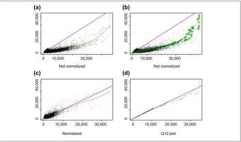
Normalization of gene expression levels between arrays. (a)The CEL intensities (see text) of a pair of replicate arrays (array 11 and 12 in array set 5) are plotted against each other. The baseline array 11 (shown on the y-axis) is not as bright as array 12 (shown on the x-axis). The smoothing spline (green curve) deviates from the diagonal line y = x(blue curve), indicating the need for normalization. (b)The same plot as (a) with superimposed circles representing the invariant set, on the basis of which a piecewise linear normalization relationship is determined (black dotted line, whose y-coordinate is the normalized value of array 12). The normalization curve is close to the smoothing spline curve in (a) as the two arrays are replicated arrays and all probes should be invariant. (c) After normalization (y-axis is the baseline array 11, and x-axis the normalized value of array 12), the scatterplot centers around the diagonal line and the array 12 is adjusted to have the similar overall brightness as array 11. The smoothing spline curve is also close to the diagonal line. (d)The Q-Q plot of probe intensities of array 11 and normalized array 12 shows the probes in the two sets have almost the same distribution.

40,000

20,000

0 10,000

10,000 20,000 30,000 40,000

0 0 10,000 20,000 30,000 40,000

30,000

Not normalized Not normalized

Normalized Q-Q plot

0 10,000 30,000

0

40,000

20,000

0

40,000

20,000

0

40,000

20,000

0

(a)

(b)

Acknowledgements

We thank Sven de Vos, Dan Tang, Nik Brown, Stan Nelson, Jae K. Lee, Yaron Hakak, John Walker and Arindam Bhattacharjee for providing data, and the editor and referees who provided valuable suggestions. This work is supported in part by NIH grant 1 RO1 HG02341-01 and NSF grant DBI-9904701.

References

1. Li C, Wong WH: Model-based analysis of oligonucleotide arrays: expression index computation and outlier detection.

Proc Natl Acad Sci USA 2001, 98:31-36.

2. Hakak Y, Walker JR, Li C, Wong WH, Davis KL, Buxbaum JD, Haroutunian V, Fienberg AA: Genome-wide expression analy-sis reveals dysregulation of myelination-related genes in

chronic schizophrenia. Proc Natl Acad Sci USA 2001, 98:

4746-4751.

3. Wodicka L, Dong H, Mittmann M, Ho M, Lockhart D:

Genome-wide expression monitoring in Saccharomyces cerevisiae.Nat

Biotechnol1997, 15:1359-1367.

4. Wallace D: The Behrens-Fisher and Fieller-Creasy problems.

In Lecture Notes in Statistics 1, R.A.Fisher: An Appreciation. Edited by Fienberg SE, Hinkley DV. Springer-Verlag 1988, 119-147.

5. Cox, DR, Hinkley DV: Theoretical Statistics. London: Chapman and Hall, 1974.

6. Eisen M, Spellman P, Brown P, Botstein D: Cluster analysis and

display of genome-wide expression patterns.Proc Natl Acad Sci

USA1998, 95:14863-14868

7. Tamayo P, Slonim D, Mesirov J, Zhu Q, Kitareewan S, Dmitrovsky E, Lander E, Golub T: Interpreting patterns of gene expression with self-organizing maps: methods and application to

hematopoietic differentiation. Proc Natl Acad Sci USA 1999,

96:2907-2912.

8. Efron B, Tibshirani R: An Introduction to the Bootstrap. New York: Chapman & Hall/CRC, 1993.

9. Bittner M, Meltzer P, Chen Y, Jiang Y, Seftor E, Hendrix M, Rad-macher M, Simon R, Yakhinik Z, Ben-Dork A, et al.: Molecular clas-sification of cutaneous malignant melanoma by gene

expression profiling. Nature 2000,406:536-540.

10. DNA-Chip Analyzer [http://www.dchip.org]

11. Schadt EE, Li C, Su C, Wong WH: Analyzing high-density

oligonucleotide gene expression array data. J Cell Biochem

2001, 80:192-202.

comment

reviews

reports

deposited research

interactions

information

refereed research

Figure 10

Similar plots as in Figure 9 for arrays hybridized to two different samples (array 24 and 36 of array set 5). (a) CEL intensities; (b)same plot as in (a) with superimposed circles representing the invariant set; (c) after renormalization; (d) Q-Q plot of normalized probe intensities. Note that the smoothing spline in (a) is affected by several points at the lower-right corner, which might belong to differentially expressed genes. The invariant set, on the other hand, does not include these points when determining the normalization curve, leading to a different normalization relationship at the high end.

40,000

20,000

0 10,000

10,000 20,000 30,000

0 0 10,000 20,000 30,000

30,000

Not normalized Not normalized

Normalized Q-Q plot

0 10,000 30,000

0

40,000

20,000

0

40,000

20,000

0

40,000

20,000

0

(a)

(b)