An efficient iterative scheme using family of chebyshev's operations

Research Article

An Efficient Iterative Scheme Using Family of

Chebyshev’s Operations

Seyed Hossein Mahdavi and Hashim Abdul Razak

StruHMRS Group, Department of Civil Engineering, University of Malaya, 50603 Kuala Lumpur, Malaysia

Correspondence should be addressed to Hashim Abdul Razak; [email protected]

Received 11 October 2014; Revised 18 January 2015; Accepted 19 January 2015

Academic Editor: Roman Lewandowski

Copyright © 2015 S. H. Mahdavi and H. Abdul Razak. This is an open access article distributed under the Creative Commons Attribution License, which permits unrestricted use, distribution, and reproduction in any medium, provided the original work is properly cited.

This paper presents an efficient iterative method originated from the family of Chebyshev’s operations for the solution of nonlinear problems. For this aim, the product operation matrix of integration is presented, and therefore the operation of derivative is developed by using Chebyshev wavelet functions of the first and second kind, initially. Later, Chebyshev’s iterative method is improved by approximation of the first and second derivatives. The analysis of convergence demonstrates that the method is at least fourth-order convergent. The effectiveness of the proposed scheme is numerically and practically evaluated. It is concluded that it requires the less number of iterations and lies on the best performance of the proposed method, especially for highly varying nonlinear problems.

1. Introduction

In general, one of the most popular and practical methods for the solution of nonlinear equations is iterative type schemes. The underlying concept is to linearize equations by evaluation of the nonlinear terms with known solution from the former iteration. Recently, the evaluation of iterative methods has attracted much attention due to their computational effi-ciency and feasibility in different disciplines of science and engineering. Fundamentally, these methods are developed by using Taylor series and algebraic decompositions. There are many studies conducted for improving the classical Newton’s method by introducing predictor-corrector procedures. For example, the family of Chebyshev’s methods is developed to constitute the fifth and sixth order iterative method [1– 7]. The major drawback of offered schemes is that, for corrector step of these methods, computation of the second derivative is necessary, which most of the time is excessively difficult. There have been many attempts in the literature to overcome aforementioned shortcoming for improving these methods by making relevant algorithms free from the second derivatives [3–5]. It is shown that the rate of convergence of

the modified iterative methods varies according to operation of various parameters [6,7].

Mathematically, orthogonal polynomials are widely employed for functional interpolation and approximation. The basic principle lies on interpolating a function by using prescribed fix points (known as knots). Basically, it is a bad idea to increase the number of inside knots in order to get accurate results (for the higher degree interpolations); however, implementation of the superior Chebyshev functions is only option for higher degree approximations (in referring to the Runge phenomenon) [5,8]. In practice, functional approximation using orthogonal polynomials has been received considerable attention in dealing with solution of partial, ordinary, or fractional differential equations [9]. The main property of such series is that it converts these problems to those of solving a system of linear algebraic equations, where the repeated and redundant calculations are neglected during the process of analysis, thus making the very easy solution procedure. One of the powerful tools constructed by developed versions of orthogonal polynomials is established as wavelet functions. Considerably, the effective characteristics of wavelets such

as localization properties and multiresolution analysis have been the focus of considerations among researchers. There are several studies available for application of this powerful tool in dynamical problems [10, 11] and integral equations [12, 13]; however, there are less reports received in the literature for development of iterative methods.

Subsequently, the main contribution of this paper is to develop an operation of derivative stemmed from the particular properties of Chebyshev wavelets capable of the modification of Chebyshev’s iterative methods. The structure of this paper is organized as follows. In the next section, the background of Chebyshev operations as well as the first and second kind of Chebyshev polynomials, the construction of corresponding wavelet functions, and the product matrix of integration and its well-known iterative method are briefly summarized. In Section 3 of this paper, the operation of derivative of Chebyshev is improved to approximate the first and the second derivatives.Section 4is devoted to the proposed iterative method and analysis of convergence of the least scale of wavelet functions. For this purpose, the applica-bility and feasiapplica-bility of the proposed method are investigated on two nonlinear scalar functions. Finally, two practical examples are given to validate and demonstrate efficiency and capability of the proposed method with emphasis on the solution of the geometrically nonlinear systems and highly varying nonlinear problems.

2. A Brief Background of Family of

Chebyshev Operations

In the following section, a brief background of Chebyshev wavelets of the first and second kind is presented. Basically, a family of continues wavelet functions is constructed from transformation of stretched and compressed variants of the mother wavelet𝜓(𝑥)defining as follows [14]:

𝜓_𝑎,𝑏(𝜏) = |𝑎|−0.5𝜓 (𝜏 − 𝑏

𝑎 ) , 𝑎, 𝑏 ∈R, 𝑎 ̸= 0. (1)

In this definition, 𝑎and 𝑏 represent the transition and scale of the mother wavelet 𝜓(𝑥). In general, wavelets those structured with different orders of polynomials (i.e., Chebyshev polynomials) have four underlying arguments of

𝜓𝑎,𝑏 = 𝜓(𝑘, 𝑛, 𝑚, 𝜏). Any positive integer𝑘is the parameter

of transition,𝑛indicates the corresponding scale,𝑚is the degree (order) of the relevant polynomials, and𝜏denotes the local coordinate of the wavelet. Fundamentally, a function is approximated by transition of scaled wavelets on the global interval of𝑥_𝑖 to𝑥_𝑖+1 (𝑖 = 0, 1, 2, . . .). This global interval is dividing into the many subdivisions according to the degree of the corresponding wavelet. The idea of discretizing the global domain into the multiple partitions appropriate to the global-scaled-frequency analysis is known as Segmentation Method (SM) [10]. The main purpose of SM is to define several collocation points on the main setting domain (global points of 𝑥_𝑖 along the global domain) and therefore to convey components of those to the new alternative domain of the analysis (i.e., local points𝜏_𝑖in frequency domain). In this study, 2𝑘−1𝑀 is assumed as the number of partitions

in each global interval (in referring to the SM collocation points) and the corresponding wavelets are constructed by

𝑚 = 0, 1, 2, . . . , (2𝑘−1𝑀/2𝑘−1) − 1order of the considered

polynomials. Accordingly, local coordinates of𝜏_𝑖are defined based on SM as follows:

𝜏𝑖= (_2𝑘−11_𝑀) (𝑖 − 0.5) , 𝑖 = 1, 2, 3, . . . , 2𝑘−1𝑀. (2)

Clearly, for mapping the coordinates of interval[0, 1]to [𝑥_𝑖, 𝑥_𝑖+1] one may use𝑥_2𝑀 = 𝑥_𝑖+ 𝜏_𝑖(𝑥_𝑖+1− 𝑥_𝑖). It should be noted that, in this study,𝑘 = 2is assumed for all derivations and calculations.

2.1. The First Kind of Chebyshev Wavelet. The families of orthogonal Chebyshev polynomials are classified into two main types. The first kind of Chebyshev polynomials𝑇_𝑚(𝑥) is obtained by a recursive formulation as follows [5,15,16]:

𝑇₀(𝑥) = 1, 𝑇₁(𝑥) = 𝑥,

𝑇_𝑚+1(𝑥) = 2𝑥𝑇_𝑚(𝑥) − 𝑇_𝑚−1(𝑥) , 𝑚 = 1, 2, . . . , (3)

where the orthogonality of 𝑇_𝑚(𝑥) is satisfied with respect to the weight function of 𝜔(𝑥) = 1/√1 − 𝑥2 on |𝑥| < 1. Subsequently, Chebyshev wavelets of the first kind (FCW) are constructed by substituting𝑇_𝑚(𝑥)in(1)as [14,16]

𝜓_𝑛,𝑚(𝑥)

={_{

{

(2𝑘/2) ⋅ ̃𝑇𝑚(2𝑘𝑥 − 2𝑛 + 1) , 𝑛 − 1_2𝑘−1 ≤ 𝑥 < _2𝑘−1𝑛

0, Otherwise,

(4)

where

̃𝑇𝑚(𝑥) =

{ { { { { { { { {

1

√𝜋, 𝑚 = 0,

√ 2

𝜋𝑇𝑚(𝑥) , 𝑚 > 0,

(5)

where 𝑚 = 0, 1, 2, . . . , 𝑀 − 1 and 𝑛 = 1, 2, . . . , 2𝑘−1 represent the order of corresponding polynomials and the considered scale of the wavelet, respectively.𝑇_𝑚(𝑥)shows the recursive formula in(3)relevant to the different orders of𝑚. Subsequently, dilated and transformed weight functions of

𝜔(𝑥)are obtained as𝜔_𝑛(𝑥) = 𝜔(2𝑘𝑥 − 2𝑛 + 1)to calculate orthogonal Chebyshev wavelets of the first kind (FCW).

2.2. The Second Kind of Chebyshev Wavelet. Chebyshev poly-nomials of the second kind 𝑈_𝑚(𝑥) are expressed by the recurrence relation of [5]

𝑈₀(𝑥) = 1, 𝑈₁(𝑥) = 2𝑥,

𝑈_𝑚+1(𝑥) = 2𝑥𝑈_𝑚(𝑥) − 𝑈_𝑚−1(𝑥) , 𝑚 = 1, 2, . . . . (6)

The weight functions of 𝜔(𝑥) = (2/𝜋)√1 − 𝑥2, (|𝑥| <

𝑈_𝑚(𝑥). The second kind of Chebyshev wavelets (SCW) is constituted as follows [17]:

𝜓_𝑛,𝑚(𝑥)

={{_{{

{

(2𝑘/2_{) ⋅ ̃𝑈}

𝑚(2𝑘𝑥 − 2𝑛 + 1) , 𝑛 − 1₂𝑘−1 ≤ 𝑥 <

𝑛

2𝑘−1,

0, Otherwise,

(7)

where𝑈̃_𝑚(𝑥) = √2/𝜋𝑈_𝑚(𝑥)and arguments of𝑘, 𝑛, and𝑚are the same as presented before. In addition, for different orders of𝑚,𝑈_𝑚(𝑥)is obtained from(6). Correspondingly, delayed and transitioned weight functions of𝜔_𝑛(𝑥) = 𝜔(2𝑘𝑥 − 2𝑛 + 1) are developed to calculate orthogonal SCWs.

2.3. Functional Decomposition. Mathematically, any quadrat-ically integrable function 𝑓(𝑥)may be decomposed by the truncated series of a wavelet’s family (i.e., FCW or SCW) as follows [13,14,17]:

𝑓 (𝑥) ≅2

𝑘−1 ∑ 𝑛=1 𝑀−1 ∑ 𝑚=0

𝑐_𝑛,𝑚𝜓_𝑛,𝑚(𝑥) = 𝐶𝑇Ψ (𝑥) , (8)

where𝐶denotes the vector of coefficients of the considered wavelets, that is, FCW or SCW. Furthermore,Ψ(𝑥)represents the vector of corresponding wavelet functions defined as

𝐶 = [𝑐₁, 𝑐₂, 𝑐₃, . . . , 𝑐₂𝑘−1]𝑇₂𝑘−1_𝑀×1

⇐⇒ 𝑐_𝑖= [𝑐_𝑖0, 𝑐_𝑖1, 𝑐_𝑖2, . . . , 𝑐_{𝑖,𝑀−1}]𝑇,

𝑖 = 1, 2, . . . , 2𝑘−1,

Ψ (𝑥) = [𝜓1, 𝜓2, 𝜓3, . . . , 𝜓2𝑘−1]𝑇₂𝑘−1_𝑀×1

⇐⇒ 𝜓_𝑖(𝑥) = [𝜓_𝑖0(𝑥) , 𝜓_𝑖1(𝑥) , 𝜓_𝑖2(𝑥) , . . . , 𝜓_{𝑖,𝑀−1}(𝑥)]𝑇.

(9)

Eventually, a 2𝑘−1𝑀 × 2𝑘−1𝑀-dimensional matrix of

𝜙_𝑛,𝑚(𝑥)is developed as

𝜙_𝑛,𝑚(𝑥) = [Ψ (𝑥1) Ψ (𝑥2) ⋅ ⋅ ⋅ Ψ (𝑥𝑖)]2𝑘−1_𝑀×2𝑘−1_𝑀. (10)

The square matrix of𝜙_𝑛,𝑚(𝑥)is populated with vectors of wavelet functions for a set of discrete SM local points (𝑥_𝑖,𝑖 =

1, 2, 3, . . . , 2𝑘−1_𝑀).

2.4. Product Matrix of Integration. The product matrix𝑃of integration (for FCW and SCW) is briefly discussed in this section. The detailed calculations of𝑃can be found in [14,17]. Assumption of the integration ofΨ(𝑥)is as follows (for𝑘 =

2):

∫1

0 Ψ2𝑀(𝑥) 𝑑𝑡 = 𝑃2𝑀Ψ (𝑥) . (11)

In(11), the subscripts ofΨ_2𝑀and𝑃_2𝑀denote the dimen-sion of matrices. Accordingly, the2𝑘𝑀 × 2𝑘𝑀-dimensional operational matrix𝑃for FCW and SCW is derived as

𝑃 = 1

2𝑘 [ [ [ [ [ [ [ [ [ [ [

[𝐿]_𝑀×𝑀 [𝐹]_𝑀×𝑀 𝐹 ⋅ ⋅ ⋅ 𝐹

[𝑂]𝑀×𝑀 [𝐿]𝑀×𝑀 𝐹 ⋅ ⋅ ⋅ 𝐹

𝑂 𝑂 d d ...

... ... ⋅⋅⋅ d 𝐹

𝑂 𝑂 ⋅ ⋅ ⋅ 𝑂 𝐿

] ] ] ] ] ] ] ] ] ] ] , (12)

where𝑀 × 𝑀square matrices𝐹and𝐿are given as follows:

𝐹 = [ [ [ [ [ [ [ [ [ [ [ [ [ [

2 0 0 ⋅ ⋅ ⋅ 0 0 0 0 0 ⋅ ⋅ ⋅ 0 0

𝑎₁ 0 0 ⋅ ⋅ ⋅ 0 0

0 0 0 d ... ...

... ... ... ... d ...

𝑎₂ 0 ⋅ ⋅ ⋅ ⋅ ⋅ ⋅ 0 0

] ] ] ] ] ] ] ] ] ] ] ] ] ] , 𝐿 = [ [ [ [ [ [ [ [ [ [ [ [ [ [ [ [ [ [ [ [ [

1 𝑎₆ 𝑎₉ 𝑎₁₂ ⋅ ⋅ ⋅ 0 0 0

𝑎₃ 0 𝑎₁₀ 𝑎₁₃ ⋅ ⋅ ⋅ 0 0 0

𝑎₄ 𝑎₇ 0 𝑎₁₄ ⋅ ⋅ ⋅ 0 0 0

𝑎₅ 𝑎₈ 𝑎₁₁ 0 ⋅ ⋅ ⋅ ... ... ...

... ... ... ... d ... ... ...

... ... ... ... ... d ... ...

𝑎15 0 0 ⋅ ⋅ ⋅ ⋅ ⋅ ⋅ 𝑎17 d 𝑎19

𝑎₁₆ 0 0 ⋅ ⋅ ⋅ ⋅ ⋅ ⋅ 0 𝑎₁₈ 0

] ] ] ] ] ] ] ] ] ] ] ] ] ] ] ] ] ] ] ] ] . (13)

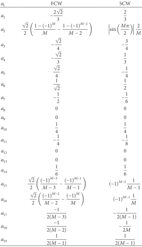
It is deduced from (12) and(13) that the population of arrays of𝑃is similar for FCW and SCW. In detail, coefficients of𝑎_𝑖are defined for FCW and SCW and tabulated inTable 1 [14,17].

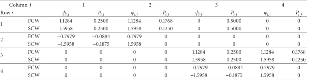
It is to be pointed out that 𝑀refers to2𝑘−1𝑀/2𝑘−1. To calculate product matrix of𝑃for FCW and SCW, a backward algorithm of program coding is recommended. In other words, only the first four rows and columns of𝑃are being computed, initially. Then, the elements of𝑃being calculated from the last row and column𝑀th until computation of the 5th row and column. To clarify the expression of wavelet’s parameters of FCW and SCW, matrices of𝜙_4,4and𝑃_4,4are calculated and tabulated inTable 2for𝑘 = 2,𝑀 = 2.

The practical effectiveness of data displayed inTable 2will be discussed in detail later.

Table 1: Coefficients of𝑎_𝑖, defined in(13)corresponding to FCW and SCW.

𝑎𝑖 FCW SCW

𝑎1 −2√2₃ 2₃

𝑎2 √2₂ (1 − (−1) 𝑀

𝑀 −1 − (−1)

𝑀−2

𝑀 − 2 ) 󵄨󵄨󵄨󵄨󵄨󵄨󵄨sin( 𝑀𝜋

2 )󵄨󵄨󵄨󵄨󵄨󵄨󵄨 2 𝑀

𝑎₃ −√2

4 −

3 4

𝑎₄ −√2

3

1 3

𝑎5 √2₄ −1₄

𝑎₆ 1

√2

1 2

𝑎7 −1₂ −1₆

𝑎8 0 0

𝑎₉ 0 0

𝑎₁₀ 1

4

1 4

𝑎11 −1₄ −1₈

𝑎₁₂ 0 0

𝑎13 0 0

𝑎₁₄ 1

6

1 6 𝑎15 √2₂ ( (−1)

𝑀−3

𝑀 − 3 − (−1)

𝑀−1

𝑀 − 1 ) (−1)𝑀−2

1 𝑀 − 1

𝑎16 √2₂ ( (−1) 𝑀−2

𝑀 − 2 − (−1)

𝑀

𝑀 ) (−1)𝑀−1

1 𝑀

𝑎17 _{2(𝑀 − 3)}−1 −_{2(𝑀 − 1)}1

𝑎18 _{2(𝑀 − 2)}−1 −_2𝑀1

𝑎₁₉ 1

2(𝑀 − 1)

1 2(𝑀 − 1)

This scheme converges quadratically and for a single nonlin-ear equation is expressed as𝑥_𝑛+1 = 𝑥_𝑛 − 𝑓(𝑥_𝑛)/𝑓󸀠(𝑥_𝑛)[2– 4]. One of the iterative methods utilized to improve New-ton’s scheme lies on the third-order convergent Chebyshev’s method. According to this algorithm, the new point of𝑥_𝑛+1 is iterated from the preceding point of𝑥_𝑛by [7]

𝑥_𝑛+1= 𝑥_𝑛− (1 + 1

2

𝑓󸀠󸀠_(𝑥

𝑛) 𝑓 (𝑥𝑛)

𝑓󸀠_(𝑥

𝑛) )

𝑓 (𝑥_𝑛)

𝑓󸀠_(𝑥

𝑛).

(14)

As it is shown in(14), iterative Chebyshev’s algorithm is rigorously dependent on the calculation of second deriva-tives, in which most of the time it is neither possible nor practical. Thus, the computing process is excessively diffi-cult, and therefore the practical applications are extremely restricted, particularly, for solving highly varying nonlinear systems. Consequently, the main contribution of our study is discovered here, whereby an iterative procedure is proposed

to improve (14) by employing FCW and SCW free from computation of the second derivatives.

3. The Proposed Method for Operation

of Derivative

In this section, an efficient approach is proposed for approx-imation of derivatives using free-scaled wavelet functions. The proposed method is applicable for various wavelet basis functions, once the product matrix of integration and wavelet coefficient vectors are available. For this purpose, integral functions are numerically developed from local coordinates to global system. For a differentiable function of𝑓(𝑥):𝑥 ∈

[𝑥_𝑛, 𝑥_𝑛+1], indefinite formulation of(15)is considered based on the Newton theorem as follows:

𝑓 (𝑥) = 𝑓 (𝑥𝑛) + ∫

𝑥

𝑥𝑛

𝑓󸀠(𝑥) 𝑑𝑥. (15)

We initialize𝑥_𝑛+1 = 𝑥_𝑛− 𝑓(𝑥_𝑛)/𝑓󸀠(𝑥_𝑛)for definite form of(15); let𝑑_𝑛= 𝑥_𝑛+1− 𝑥_𝑛. Using(8)the derivative function is approximated on global coordinates as follows:

𝑓󸀠(𝑥) = 𝐶𝑇⋅ Ψ (𝑥) . (16)

Substituting into(15)we have

𝑓 (𝑥_𝑛+1) = 𝑓 (𝑥_𝑛) + ∫𝑥𝑛+1

𝑥𝑛

𝐶𝑇⋅ Ψ (𝑥) 𝑑𝑥. (17)

Multiplying by operational matrix 𝑃 of integration, adding initial constant of integration, we have

𝑓 (𝑥_𝑛+1) = 𝑓 (𝑥_𝑛) + 𝑑_𝑛⋅ 𝐶𝑇_{⋅ 𝑃 ⋅ Ψ (𝑥) + 𝑓}󸀠_(𝑥

0) , (18) where 𝑑_𝑛 is operated for mapping local characteristics of Chebyshev wavelet to global ones. To simplify this equation, constant quantities are approximated by Chebyshev wavelets in each step. For this purpose, the unity is being expanded by the Chebyshev wavelet as [10,15,16]

1 ≅ 𝐼∗Ψ (𝑡) ≅ 𝐷 [11,1, 0, 0, . . . , 11,𝑀+1, 0, 0, . . .] Ψ (𝑡) , (19)

where 𝐷 = √𝜋/4and √𝜋/8for FCW and SCW, respec-tively. Therefore, initial values are developed as2𝑘−1𝑀 × 1 -dimensional vectors corresponding to collocation points:

𝑓󸀠(𝑥₀) = 𝑓󸀠(𝑥₀) 𝐼∗Ψ (𝑥) ,

𝑓 (𝑥_𝑛+1) = 𝑓 (𝑥_𝑛+1) 𝐼∗Ψ (𝑥) ,

𝑓 (𝑥𝑛) = 𝑓 (𝑥𝑛) 𝐼∗Ψ (𝑥) .

(20)

Substituting(20)into(18)we have

𝑓 (𝑥𝑛+1) 𝐼∗Ψ (𝑥) = 𝑓 (𝑥𝑛) 𝐼∗Ψ (𝑥) + 𝑑𝑛⋅ 𝐶𝑇⋅ 𝑃

⋅ Ψ (𝑥) + 𝑓󸀠(𝑥₀) 𝐼∗Ψ (𝑥) . (21)

Table 2: Corresponding components of wavelets𝜙_𝑖,𝑗and𝑃, calculated on four SM = 4 points for FCW and SCW.

Column𝑗 1 2 3 4

Row𝑖 𝜙_𝑖,𝑗 𝑃_𝑖,𝑗 𝜙_𝑖,𝑗 𝑃_𝑖,𝑗 𝜙_𝑖,𝑗 𝑃_𝑖,𝑗 𝜙_𝑖,𝑗 𝑃_𝑖,𝑗

1 FCW 1.1284 0.2500 1.1284 0.1768 0 0.5000 0 0

SCW 1.5958 0.2500 1.5958 0.1250 0 0.5000 0 0

2 FCW −0.7979 −0.0884 0.7979 0 0 0 0 0

SCW −1.5958 −0.1875 1.5958 0 0 0 0 0

3 FCW 0 0 0 0 1.1284 0.2500 1.1284 0.1768

SCW 0 0 0 0 1.5958 0.2500 1.5958 0.1250

4 FCW 0 0 0 0 −0.7979 −0.0884 0.7979 0

SCW 0 0 0 0 −1.5958 −0.1875 1.5958 0

Note: FCW = first Chebyshev wavelet, SCW = second Chebyshev wavelet.

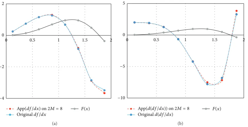
(16),𝑓󸀠(𝑥)is approximated on2𝑀global points. The same approach is employed on 𝑓󸀠(𝑥) to compute the second derivative of𝑓󸀠󸀠(𝑥). The proposed method is implemented on

𝑓(𝑥) = sin(𝑥2);𝑥 ∈ [0, 2], in which its definite𝑓󸀠(𝑥) = 2𝑥 ⋅

cos(𝑥2)and𝑓󸀠󸀠(𝑥) = 2[cos(𝑥2) − 2𝑥2sin(𝑥2)]exist. The first

and second derivatives are calculated for2𝑀 = 8collocation points of FCW and SCW and have been compared with exact values (designated by original𝑑𝑓/𝑑𝑥or𝑑(𝑑𝑓/𝑑𝑥)) in Figures 1and 2, respectively. The approximated results for the first and second derivatives of𝑓(𝑥)are designated in figures by

App(𝑑𝑓/𝑑𝑥) and App(𝑑(𝑑𝑓/𝑑𝑥)), respectively.

The schematic view of results in Figures1and2lies on the better accuracy of SCW, when2𝑀 = 8is applied. For the purpose of a detailed comparison, various2𝑀points are employed through the proposed method corresponding to diverse scales of FCW and SCW to calculate the first and second derivative of considered 𝑓(𝑥). The comparison of results is depicted in Figures3and4related to the FCW and SCW, respectively. Accordingly, the percentile total average error (PTAE) measurement is presented for the purpose of comparison. By assumption of𝛼for the closed-form solution and𝑋_𝑐as the calculated value, PTAE is defined as PTAE =

100 ∑ |(𝛼 − 𝑋_𝑐)/𝛼|.

The measured PTAE data shown in Figures 3 and 4 illustrate that free scales of SCW approximate the first and second derivatives more accurate than those of FCW. For instance, PTAE = 89.49% is measured for the second scale of FCW, while this value is considerably decreased to 9.32% for the same scale of SCW. As it is shown in Figure 3, the accuracy of the second derivative is more than the first one. This is because the oscillatory shape of the results coincides with the exact result for the second derivative, in contrast to the calculated results by SCW for the first derivative. Significantly, the error measurement of the proposed method using higher scales of SCW demonstrates the superiority of this wavelet. Finally, it is apparent from the figures that end point errors diversely affect the accuracy of results for the higher order approximations shown for2𝑀= 64 collocation points.

In addition, the proposed scheme is applicable in prob-lems with several unknowns, where the tangent line becomes

a tangent (hyper) plane. For instance,(15)is developed for a function of two variables𝑓(𝑥, 𝑦)as follows:

𝑓 (𝑥, 𝑦 = 𝑦₀) = 𝑓 (𝑥_𝑛, 𝑦 = 𝑦₀) + ∫𝑥

𝑥𝑛

𝑓󸀠

𝑥(𝑥, 𝑦 = 𝑦0) 𝑑𝑥,

(22)

where𝑥and𝑦 = 𝑦₀represent the first variable and the con-stant point for the second variable, respectively.𝑓_𝑥󸀠(𝑥, 𝑦 = 𝑦₀) indicates the derivative of 𝑓(𝑥, 𝑦)with respect to 𝑥 while

𝑦 = 𝑦0and the subscripts𝑥and𝑦are changed for the next

variable as

𝑓 (𝑥 = 𝑥₀, 𝑦) = 𝑓 (𝑥 = 𝑥₀, 𝑦_𝑛) + ∫𝑦

𝑦𝑛

𝑓_𝑦󸀠(𝑥 = 𝑥₀, 𝑦_𝑛) 𝑑𝑦.

(23)

Consequently,𝑓_𝑥󸀠and𝑓_𝑦󸀠are calculated, and therefore the normal vector ( ⃗𝑛) to the plane at𝑥₀and𝑦₀is derived as

⃗𝑛 = ⟨𝑓_𝑥󸀠(𝑥₀, 𝑦₀) , 𝑓_𝑦󸀠(𝑥₀, 𝑦₀) , −1⟩ . (24)

4. The Proposed Iterative Method

The proposed iterative method contains the set of modi-fied predictors-correctors explained in (14). The operation of derivative proposed in previous section is employed to approximate the second derivatives using FCW and SCW. Basically, the most accurate results are computed for the approximation of only the second derivative; however, the method is also applicable for approximation of the first derivative. For this purpose,𝑦_𝑛= 𝑥_𝑛−𝑓(𝑥_𝑛)/𝑓󸀠(𝑥_𝑛)is initially predicted. Later, the second derivatives of 𝑓(𝑥) for 𝑥 ∈

0 1 2

0 0.5 1 1.5 2

App(df/dx) on2M = 8

Originaldf/dx

F(x) −1

−2

−3

−4

(a)

0 2 4

0 0.5 1 1.5 2

F(x)

Originald(df/dx) −2

−4

−6

−8

−10

App(d(df/dx))on2M = 8

(b)

Figure 1: The approximated results using the proposed operation of derivative of FCW on2𝑀= 8 collocation points for calculation of (a) the first and (b) the second derivative.

Original_df/dx

F(x)

0 2

−2

−4

0 0.5 1 1.5 2

App(df/dx) on2M = 8

(a)

F(x)

Original_d(df/dx) 0

5

−5

−10

0 0.5 1 1.5 2

App(d(df/dx))on2M = 8

(b)

Figure 2: The approximated results using the proposed operation of derivative of SCW on2𝑀= 8 collocation points for computation of (a) the first and (b) the second derivative.

0 50 100

PT

AE (%)

First derivative Second derivative

2M2 _2M4

2M8 _2M16

2M32 _2M64

2M2, 11.04 2M4, 10.71

2M8, 9.29 2M16, 3.66

2M32, 0.68 _{2M64, 1.28}

Figure 3: PTAE measurement corresponding to different scales (2𝑀collocations) of FCW.

PT

AE (%)

First derivative Second derivative 0

10 20

2M2 _2M4

2M8 _2M16

2M32 _2M64

2M2, 11.06 2M4, 6.99

2M8, 4.23 2M16, 0.195

2M32, 2.41E − 07 2M64, 1.41E − 05

row of matrix𝑃and vector𝐶as (the matrix calculus is then satisfied):

𝑥_𝑛+1= 𝑥_𝑛− (1 +1

2

𝐶𝑇_{𝜓 (𝑥) ⋅ 𝐶}𝑇_𝑃2_{𝜓 (𝑥)}

𝐶𝑇_{𝑃𝜓 (𝑥)} )

𝑓 (𝑥_𝑛)

𝑓󸀠_(𝑥

𝑛). (25)

Using(7)and substituting𝜓_1,1(𝑥) = (√2/𝜋)(16𝑥 − 4)for SCW yield

𝑥𝑛+1= 𝑥𝑛− (1 +1₂𝜂 (16𝑥𝑛− 4))_𝑓𝑓 (𝑥_󸀠(𝑥𝑛)

𝑛), (26)

where𝜂is assumed as an independent variable of the error function. On the other hand, let𝛼 be a simple root of𝑓;

thus𝑓(𝛼) = 0and𝑓󸀠(𝛼) ̸= 0. As long as𝑓is a sufficiently

differentiable function, using Taylor series expansion of𝑓and

𝑓󸀠_around𝑥

𝑛= 𝛼gives [1–4,8]

𝑓 (𝑥_𝑛) = 𝑓󸀠(𝛼) (𝑥_𝑛− 𝛼) + 1

2!𝑓󸀠󸀠(𝛼) (𝑥𝑛− 𝛼)

2

+ 1

3!𝑓󸀠󸀠󸀠(𝛼) (𝑥𝑛− 𝛼)

3_{+ ⋅ ⋅ ⋅ + 𝑂 ((𝑥}

𝑛− 𝛼)4) . (27)

Using𝑂(𝑒_𝑛𝑙) = ∑∞_𝑖=𝑙𝑐_𝑖𝑒_𝑛𝑖and𝑐_𝑠= (1/𝑠!)(𝑓𝑠(𝛼)/𝑓󸀠(𝛼)),𝑠 =

1, 2, . . .and𝑒_𝑛= 𝑥_𝑛−𝛼,(27)is therefore developed as follows:

𝑓 (𝑥_𝑛) = 𝑓󸀠(𝛼) [𝑒𝑛+ 𝑐2𝑒𝑛2+ 𝑐3𝑒𝑛3

+ 𝑐₄𝑒_𝑛4+ 𝑐₅𝑒_𝑛5+ ⋅ ⋅ ⋅ + 𝑂 (𝑒_𝑛6)] . (28)

Accordingly, the first derivative of𝑓is obtained as

𝑓󸀠(𝑥_𝑛) = 𝑓󸀠(𝛼) [1 + 2𝑐₂𝑒_𝑛+ 3𝑐₃𝑒_𝑛2

+ 4𝑐₄𝑒_𝑛3_{+ 5𝑐}

5𝑒𝑛4+ ⋅ ⋅ ⋅ + 𝑂 (𝑒𝑛5)] .

(29)

Dividing(28)by(29), one may obtain

𝑓 (𝑥_𝑛)

𝑓󸀠_(𝑥

𝑛) = 𝑒𝑛− 𝑐2𝑒𝑛

2_{+ 2 (𝑐}2

2− 𝑐3) 𝑒𝑛3+ ⋅ ⋅ ⋅ + 𝑂 (𝑒𝑛4) .

(30)

Let𝑒_𝑛= 𝑥_𝑛− 𝛼; therefore,(26)is developed as follows:

𝑥_𝑛+1= 𝑥_𝑛− (1 +1

2𝜂 (16𝑒𝑛+ 16𝛼 − 4))

⋅ [𝑒_𝑛− 𝑐₂𝑒_𝑛2+ 2 (𝑐₂2− 𝑐₃) 𝑒_𝑛3+ ⋅ ⋅ ⋅ + 𝑂 (𝑒_𝑛4)] .

(31)

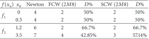
Table 3: Comparison of the proposed iterative methods and Newton’s method for solution of𝑓₁and𝑓₂.

𝑓(𝑥𝑛) 𝑥0 Newton FCW (2𝑀8) 𝐷% SCW (2𝑀8) 𝐷%

𝑓₁ 0 4 2 50% 2 50%

0.5 4 2 50% 2 50%

𝑓₂ 1.2 6 2 66.7% 2 66.7%

3.5 7 4 42.85% 3 57.14%

Note: FCW (2𝑀8), SCW (2𝑀8) = first and second kind of Chebyshev wavelets on2𝑀 = 8.

This means that the order of convergence of the proposed method is at least four (𝑒_𝑛4), when the least scale of SCW is employed. The same approach is applied for FCW and the same convergence rate is obtained.

Now we present two examples to investigate the efficiency of the improved iterative method. The solution of two scalar nonlinear equations𝑓₁(𝑥)and𝑓₂(𝑥)is considered as follows:

𝑓₁(𝑥) = 𝑥2− 𝑒𝑥− 3𝑥 + 2, 𝛼 = 0.2575302854,

𝑓₂(𝑥) =sin2(𝑥) − 𝑥2+ 1, 𝛼 = 1.4044916482,

(32)

where𝛼 denotes the simple root of the nonlinear equation and the prescribed error measurement at the ending of the iteration process is |𝑓(𝑥_𝑛)| < 1 ⋅ 𝑒 − 6. The total number of iterations (NIt) and relative percentile reduction of NIt (designated by𝐷%) from the starting point of𝑥_𝑛are compared for the classical Newton’s method and the proposed methods of FCW and SCW (for2𝑀 = 8), shown inTable 3.

Obviously, data displayed in Table 3 demonstrate that FCW and SCW require lesser number of iterations than Newton’s method. In addition, it shows the satisfactory performance of the developed method using2𝑀 = 8scales of FCW, while the superior performance is observed for SCW.

5. Numerical Application

One of the important practices of iterative methods is nonlinear structural analysis. In structural analysis,{𝑓(𝑥)} =

𝑃is the equilibrium equation of structural elements with the vector of nodal internal loadings{𝑓} subjected to external forces 𝑃. In a nonlinear structure, the load-deformation relations of each degree of freedom (DOF) illustrate that

{𝑓}is a nonlinear function of displacements{𝑥}. Therefore, the convenient analysis will be carried out by using the incremental form of structural equilibrium of[𝐾_𝑡] {Δ𝑥} =

ΔP

n

=Δ

Qn _[KPredicted

t ]

[KtPredicted] [K

Corrected

t ]

[KtCorrected]

Newton’s method Proposed method

xny1 · · · yn

ΔQn+1

Displacement (x)

xn+1

y2M

Load (P)

Figure 5: The geometric construction of the proposed method using FCW or SCW.

Undeformed shape

l =l0

𝛽

a

P

Δ

h

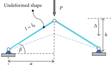
Figure 6: William’s toggle frame subjected to the𝑃at the apex.

describes the overall process of Newton-Raphson method and the proposed method, whereby the out-of-balanced force

Δ𝑄_𝑛is considered for new iterations (correctors).

The geometrically nonlinear analysis of the well-known William’s toggle frame is considered in this section.Figure 6 shows the geometry of this simple frame comprised of two truss elements and one DOF.𝐸=20.7𝑒3N/cm2, 𝐴= 1 cm2, and𝑙= 254 cm are chosen as the modulus of elasticity, cross-sectional area, and undeformed length, respectively. The load increment ofΔ𝑃 = 550kN is applied at the top node of this truss for two increments(𝛽 = 30∘).

In this application, the displacement-control criterion is utilized to stop the ending iterations and the tolerance factor

1𝑒 − 3 is accordingly chosen. Basically, the geometrically

nonlinear equilibrium and the one DOF tangential stiffness [𝐾_𝑡] of this structure (which is the gradient of the𝑓(𝑥)) are defined as [18]

𝑓 (𝑥) = 2𝐸𝐴 (sin(𝛽) − Δ

𝑙)

⋅ [[

[

1

√1 + (Δ/𝑙)2_{− 2 (Δ/𝑙)sin(𝛽)} − 1]]

] ,

𝐾_𝑡= 1 − cos2(𝛽)

(1 + (Δ/𝑙)2− 2 (Δ/𝑙)sin(𝛽))1.5.

(33)

This structure is analyzed using the proposed method of FCW and SCW (2𝑀 = 8) and the classical Newton’s method for two increments of load. For the classical Newton’s

Table 4: Comparison of number of iterations (NIt) for two incre-ments ofΔ𝑃.

-FCW SCW

NIt 𝐷% NIt 𝐷%

2𝑀 = 2 32 33% 30 37%

2𝑀 = 4 30 37% 29 39%

2𝑀 = 8 29 39% 24 50%

method the convergence criteria are achieved by NIt = 48 for two increments (predictions). Subsequently, total number of iterations (NIt) and relative percentile reductions are displayed inTable 4corresponding to various scales of FCW and SCW.

It is apparent fromTable 4that the convergence criterion is accomplished by less iterations using the 8th scales of SCW. It is shown that this scale of wavelet rapidly converges. Furthermore, the competency of the proposed method is also confirmed by FCW, while it requires the less number of iterations compared with Newton’s method. Actually, the main computational efficiency of the proposed method is not discovered well through this application, where the similar number of increments is utilized for Newton’s and the pro-posed method. As a result, the computational time (recorded with a same hardware) due to the 8th scales of the proposed method reached the highest value of 0.5 sec compared with the minimum value of 0.01 sec recorded for the solution of Newton’s method. However, the best rate of convergence is achieved by the proposed method. It is concluded that the best performance of the proposed method is revealed in statically or dynamically highly varying nonlinear problems, in which the initial value of𝑓_(𝑥󸀠Predicted_𝑛) may be predicted for a long increment ofΔ𝑃as shown inFigure 7.

Figure 7shows the shortcoming of Newton’s method for the highly varying nonlinear problems. In contrast, it is illustrated that the highly varying nonlinear behaviors are accurately captured using the proposed method of FCW or SCW on corresponding collocation points. In this figure𝑥𝑤_2𝑀 refers to the2𝑀collocation points of wavelet, the same as introduced in Figure 5for initial predictions of𝑦₁ to𝑦_2𝑀. It is shown that the only increment ofΔ𝑃 applied for the proposed method will be divided to at least four increments of Newton’s scheme in pursuit of an accurate analysis (for this particular case). Consequently, the cost of analysis is significantly increased depends on existed nonlinearity. Such nonlinear behaviors cannot happen on our practical example (geometric nonlinearity of structures), where the nonlinear path is almost linear until the first critical point (inflection point). However in many applications of physics or chemistry aforementioned highly nonlinear characteristics are considered through both static and dynamic analysis.

Δx0 Δx0

f(x) f(x)

f(x󳰀Predicted𝑛)

ΔP

x

x

xn xw₁ xw₂ xw₃ xw_2M xn+1

Newton’s method Proposed

method

· · · xn xw₁ xw₂ xw₃ · · · xw_2M xn+1

ΔP4

ΔP3

ΔP2

ΔP1

f(x󳰀Predicted𝑛)

Figure 7: The geometric illustration of computational efficiency of the proposed method compared with Newton’s method.

f_(x)󳰀Predicted

f(x)󳰀Corrected

ΔP = 14 18

16 14 12 10 8 6 4 2 0

0 2 4 6 8 10 12 14 16

f(x)

xn xn+1

xw

1 x w

2x3wx4wx5wxw6 x7wx8w x

f(x) = x + (1/3) ·sin(3 · x)

Figure 8: The schematic view of iterative solution of nonlinear𝑓(𝑥) using the proposed method.

𝑓(𝑥) = 𝑥 + 𝛼Sin(𝛽𝑥),𝛼 = 1/3, and𝛽= 3 is evaluated by

Newton’s scheme and various scales of FCW and SCW. For this purpose, one increment of Δ𝑃= 14 is considered for the proposed procedure, whereas eight increments ofΔ𝑃are utilized for the classical Newton’s method to capture details of foregoing function. The schematic view of iterative solution of

𝑓(𝑥)using the proposed scheme is shown inFigure 8. As it is shown inFigure 8, by using the long increment of

Δ𝑃= 14, details of the nonlinear function are almost accu-rately evaluated to iterate new𝑥_𝑛+1from𝑥_𝑛. The prescribed error measurement at the ending of the iteration process is

|𝑓(𝑥_𝑛)| < 1 ⋅ 𝑒 − 5. The total number of iterations (NIt),

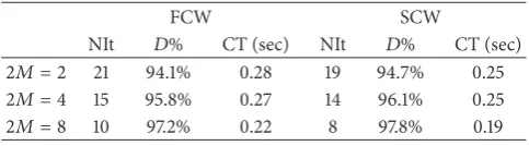
relative percentile reduction of NIt (designated by𝐷%) from the starting point of𝑥_𝑛, and computation time involved (CT) are compared inTable 5for the proposed methods of FCW and SCW. It is to be noted that NIt = 361 is recorded for the classical Newton’s method (8 numbers ofΔ𝑃) with CT = 0.53 sec.

Data inTable 5shows that the best efficiency is recorded for SCW (2𝑀 = 8) by NIt = 8 and the least time consumption of CT = 0.19 sec. It is shown that, for the low scales of FCW and SCW (2𝑀 = 2 or 4), because of the simplicity of function’s evaluation of 2𝑀 = 2, the final computational times are almost the same. However, for the larger scales, time

Table 5: Comparison of number of iterations (NIt) and computa-tional time (CT) for one increment ofΔ𝑃 = 14.

FCW SCW

NIt 𝐷% CT (sec) NIt 𝐷% CT (sec)

2𝑀 = 2 21 94.1% 0.28 19 94.7% 0.25

2𝑀 = 4 15 95.8% 0.27 14 96.1% 0.25

2𝑀 = 8 10 97.2% 0.22 8 97.8% 0.19

consumption is decreased due to less number of iterations. Finally, this numerical example demonstrates the capability of the proposed method in such applications by using larger scales, in which details of nonlinear problem are accurately captured prior to the new iterations.

6. Conclusion

Conflict of Interests

The authors declare that there is no conflict of interests regarding the publication of this paper.

Acknowledgments

The authors wish to acknowledge the financial support from the University of Malaya (UM) and Ministry of Education of Malaysia (Grant nos. FP027/2012A, PG078/2013B, and UM.C/625/1/HIR /MOHE/ENG/55).

References

[1] D. K. Babajee, M. Z. Dauhoo, M. T. Darvishi, A. Karami, and A. Barati, “Analysis of two Chebyshev-like third order methods free from second derivatives for solving systems of nonlinear equations,”Journal of Computational and Applied Mathematics, vol. 233, no. 8, pp. 2002–2012, 2010.

[2] C. Chun, “A simply constructed third-order modifications of Newton’s method,”Journal of Computational and Applied Math-ematics, vol. 219, no. 1, pp. 81–89, 2008.

[3] C. Chun and Y. Ham, “Some fourth-order modifications of Newton’s method,”Applied Mathematics and Computation, vol. 197, no. 2, pp. 654–658, 2008.

[4] J. R. Sharma, “A composite third order Newton-Steffensen method for solving nonlinear equations,”Applied Mathematics and Computation, vol. 169, no. 1, pp. 242–246, 2005.

[5] J. C. Mason and D. C. Handscomb, Chebyshev Polynomials, Chapman & Hall/CRC Press, 2003.

[6] J. Kou, Y. Li, and X. Wang, “A modification of Newton method with third-order convergence,”Applied Mathematics and Com-putation, vol. 181, no. 2, pp. 1106–1111, 2006.

[7] D. Li, P. Liu, and J. Kou, “An improvement of Chebyshev-Halley methods free from second derivative,”Applied Mathematics and Computation, vol. 235, no. 25, pp. 221–225, 2014.

[8] W. Gautschi,Numerical Analysis, Springer, Berlin, Germany, 2011.

[9] R. Askey,Orthogonal Polynomials and Special Functions, Society for Industrial and Applied Mathematics, Philadelphia, Pa, USA, 1975.

[10] S. H. Mahdavi and H. Abdul Razak, “A wavelet-based approach for vibration analysis of framed structures,”Applied Mathemat-ics and Computation, vol. 220, pp. 414–428, 2013.

[11] S. H. Mahdavi and S. Shojaee, “Optimum time history analysis of SDOF structures using free scale of Haar wavelet,”Structural Engineering and Mechanics, vol. 45, no. 1, pp. 95–110, 2013. [12] W. M. Abd-Elhameed, E. H. Doha, and Y. H. Youssri, “New

wavelets collocation method for solving second-order multi-point boundary value problems using Chebyshev polynomials of third and fourth kinds,”Abstract and Applied Analysis, vol. 2013, Article ID 542839, 9 pages, 2013.

[13] W. Swaidan and A. Hussin, “Feedback control method using Haar wavelet operational matrices for solving optimal control problems,”Abstract and Applied Analysis, vol. 2013, Article ID 240352, 8 pages, 2013.

[14] E. Babolian and F. Fattahzadeh, “Numerical solution of differ-ential equations by using Chebyshev wavelet operational matrix of integration,”Applied Mathematics and Computation, vol. 188, no. 1, pp. 417–426, 2007.

[15] S. H. Mahdavi and H. A. Razak, “A comparative study on optimal structural dynamics using wavelet functions,” Mathe-matical Problems in Engineering. In press.

[16] S. H. Mahdavi and H. A. Razak, “An indirect time integration scheme for dynamic analysis of space structures using wavelet functions,”Journal of Engineering Mechanics (ASCE), In Press. [17] Z. Li and Y. Wang, “Second Chebyshev wavelet operational

matrix of integration and its application in the calculus of variations,”International Journal of Computer Mathematics, vol. 90, no. 11, pp. 2338–2352, 2013.

Submit your manuscripts at

http://www.hindawi.com

Hindawi Publishing Corporation

http://www.hindawi.com Volume 2014

Mathematics

Hindawi Publishing Corporation

http://www.hindawi.com Volume 2014

Mathematical Problems in Engineering

Hindawi Publishing Corporation http://www.hindawi.com

Differential Equations

International Journal of

Volume 2014

Hindawi Publishing Corporation

http://www.hindawi.com Volume 2014 Hindawi Publishing Corporationhttp://www.hindawi.com Volume 2014

Hindawi Publishing Corporation

http://www.hindawi.com Volume 2014

Mathematical PhysicsAdvances in

Complex Analysis

http://www.hindawi.com Volume 2014

Optimization

Hindawi Publishing Corporation

http://www.hindawi.com Volume 2014

Combinatorics

Hindawi Publishing Corporation

http://www.hindawi.com Volume 2014 International Journal of

Hindawi Publishing Corporation

http://www.hindawi.com Volume 2014

Journal of

Hindawi Publishing Corporation

http://www.hindawi.com Volume 2014

Function Spaces

Abstract and Applied Analysis Hindawi Publishing Corporation

http://www.hindawi.com Volume 2014

International Journal of Mathematics and Mathematical Sciences

Hindawi Publishing Corporation http://www.hindawi.com Volume 2014

The Scientific

World Journal

Hindawi Publishing Corporation

http://www.hindawi.com Volume 2014

Hindawi Publishing Corporation

http://www.hindawi.com Volume 2014

Discrete Dynamics in Nature and Society

Hindawi Publishing Corporation

http://www.hindawi.com Volume 2014 Hindawi Publishing Corporation

http://www.hindawi.com Volume 2014

Discrete Mathematics

Hindawi Publishing Corporation

http://www.hindawi.com Volume 2014 Hindawi Publishing Corporationhttp://www.hindawi.com Volume 2014