Predictive modelling of human walking over a complete gait cycle

P r e d i c tiv e m o d e lli n g of h u m a n

w a l ki n g ov e r a c o m pl e t e g a i t

c y cl e

R e n , L, Jo n e s , RK a n d H o w a r d , D

h t t p :// dx. d oi.o r g / 1 0 . 1 0 1 6 /j.j bio m e c h . 2 0 0 6 . 0 7 . 0 1 7

T i t l e P r e d i c tiv e m o d e lli n g of h u m a n w al ki n g ov e r a c o m p l e t e g ai t cy cl e

A u t h o r s R e n , L, Jo n e s , RK a n d H o w a r d , D

Typ e Ar ticl e

U RL T hi s v e r si o n is a v ail a bl e a t :

h t t p :// u sir. s alfo r d . a c . u k /i d/ e p ri n t/ 2 1 0 / P u b l i s h e d D a t e 2 0 0 7

U S IR is a d i gi t al c oll e c ti o n of t h e r e s e a r c h o u t p u t of t h e U n iv e r si ty of S alfo r d . W h e r e c o p y ri g h t p e r m i t s , f ull t e x t m a t e r i al h el d i n t h e r e p o si t o r y is m a d e f r e ely a v ail a bl e o nli n e a n d c a n b e r e a d , d o w nl o a d e d a n d c o pi e d fo r n o

n-c o m m e r n-ci al p r iv a t e s t u d y o r r e s e a r n-c h p u r p o s e s . Pl e a s e n-c h e n-c k t h e m a n u s n-c ri p t fo r a n y f u r t h e r c o p y ri g h t r e s t r i c ti o n s .

Predictive Modelling of Human Walking Over a Complete Gait Cycle

Lei Ren1,2, Richard K Jones1,3 and David Howard1,2

1

Centre for Rehabilitation and Human Performance Research

2

School of Computing, Science and Engineering & 3School of Healthcare Professions

University of Salford

Corresponding Author:

Prof. David Howard

School of Computing, Science and Engineering University of Salford

Salford M5 4WT

United Kingdom Tel. 0161 295 3584 Fax. 0161 295 5575

Email [email protected]

Keywords: gait prediction, inverse dynamics, optimisation, optimal motor task

Word count (introduction through discussion): 3000

Submitted as an Original Article

Abstract

An inverse dynamics multi-segment model of the body was combined with

optimisation techniques to simulate normal walking in the sagittal plane on level

ground. Walking is formulated as an optimal motor task subject to multiple

constraints with minimisation of mechanical energy expenditure over a complete gait

cycle being the performance criterion. All segmental motions and ground reactions

were predicted from only three simple gait descriptors (inputs): walking velocity,

cycle period and double stance duration. Quantitative comparisons of the model

predictions with gait measurements show that the model reproduced the significant

characteristics of normal gait in the sagittal plane. The simulation results suggest that

minimising energy expenditure is a primary control objective in normal walking.

However, there is also some evidence for the existence of multiple concurrent

performance objectives.

Nomenclature

an

x , y _an coordinates of ankle joint centre in global reference frame

an

x&

& , &y&an linear accelerations of ankle joint centre in global reference frame

an

x

∆ relative displacement of ankle joint along x-axis in stance phase

) ( hs an

x x coordinate of ankle joint at heel strike

ft

i

x , yi coordinates of the i

th

joint centre in global reference frame

i

x& & _,

i

y&

& linear accelerations of the ith joint centre in global reference frame

j

l length of jth body segment

j

θ , ω_j, α_j angular displacement, velocity and acceleration ofbody segment

i

m mass of ith segment

i

av translational acceleration vector for the ith segment’s mass centre

ji F

v

jth resultant joint force acting on the ith segment

ei

F

v

resultant external force acting on the ith segment

gv

gravitational vector

i

I moment of inertia of the ith segment

i

θ

α

ji

M net muscle moment acting on the ith segment at the jth joint

ei

M resultant external moment acting on the ith segment

ki

M moment of the resultant joint force at the kth joint acting on the ith

segment

gi F

v

, Mgi ground reaction force and moment acting on left or right foot

i

T net muscle torque acting at ith joint

) ( 0 i

a , ak(i), ) (i k

b coefficients in Fourier series representing ith segment angle trajectory

ω

c

T walking cycle period

) (i p

ω

ω

m

a

V average walking velocity over a walking cycle

L ankle joint displacement over a walking cycle

x

µ

Introduction

Although the biomechanics of walking is well understood (McMahon, 1984; Zajac et

al., 2003a, 2003b), little is known about the neural control strategies involved. Much

of the research has been empirical, and few have focused on gait simulation (Chow

and Jacobson, 1971, Davy and Audu, 1987; Marshall et al., 1989; Yamaguchi, 1990;

Koopman, 1995; Anderson and Pandy, 2001). In predictive gait simulation,

optimisation techniques have often been employed, where muscle forces and

movements are determined by minimising a cost function.

The most popular approach to gait prediction has been to combine optimisation with

forward dynamics, probably because this coincides with the natural sequence of

neuromuscular control (Zajac and Winters, 1990; Yamaguchi, 1990, Pandy, 2001).

However, since the system differential equations must be numerically integrated, the

forward dynamics method leads to very long simulation times. In addition, realistic

initial guesses for all control inputs (e.g. muscle activations) and initial values for all

state variables (e.g. joint angular positions and velocities) are required to ensure that

reasonable gait patterns can be obtained (Pandy, 2001). This depends on the

availability of measurement data (Marshall et al., 1989; Anderson and Pandy, 2001)

In contrast, the inverse dynamics method is very efficient computationally as it does

not require numerical integration of the system differential equations. In addition,

initial values for optimisation parameters can be set without the need for measurement

data and initial values for the state variables are unnecessary. When inverse dynamics

is applied in gait prediction, simple mathematical functions are used to represent the

trajectories of the generalized coordinates (Yen and Nagurka, 1987; Koopman, 1995),

where the function coefficients are the optimisation variables.

Only a few gait predication studies have employed inverse dynamics and optimisation

(Yen and Nagurka, 1987; Channon, 1992; Koopman, 1995; Chevallereau and

Aoustin, 2001). Most of these have considered only the single support phase or

assume an instantaneous double support phase (zero duration). In addition, the foot

segment was often neglected or assumed to be flat on the floor during stance.

Moreover, additional trajectory constraints were often imposed on the segmental

motions to simplify the optimisation problem. For example, Yen and Nagurka (1987)

modelled the human skeletal system as a five-segment linkage. However, the

trajectories of the body segments were only predicted for the single stance phase, the

trunk was assumed to be upright throughout the cycle, and the model was forced to

move at a constant forward speed. Koopman (1995) employed an eight-segment

three-dimensional model to simulate normal walking over the whole gait cycle.

However, all of the motions at the hip, knee and ankle were constrained to follow

measured data or set to zero, the aim being to predict the unmeasured trunk and pelvic

In this paper, we present a combined inverse dynamics and optimisation method to

predict normal human walking. In contrast to previous studies, the model predicts a

complete gait cycle, including a normal double support phase. The foot segment is

allowed to rotate freely during stance, rather than remaining flat on the floor. In

addition, no predefined or measured trajectory constraints are imposed on segmental

motions. The gait motions and joint torques are predicted from only three simple gait

descriptors, average walking speed, cycle period and double stance duration, which

minimizes the requirements for experimental data.

Methods

The multi-segment model

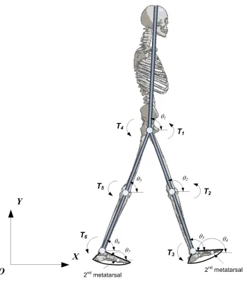
The human body was modelled as a planar (sagittal plane) seven-segment system

(Figure 1). The interaction between the foot and the floor was modelled as a rigid

contact, where the contact point is determined by the shape of the foot’s plantar

surface and the foot orientation.

Referring to Figure 1, the segmental angles

θ

θ

θ

orientation of each body segment with respect to the global reference frame. In the

double support phase, these segmental angles are not all independent because the

model becomes a closed loop mechanism. The torques T₁, T₂, …, T₆ are the net

Anthropometric data, including segment masses, centre of mass positions and

moments of inertia, are based on the data of de Leva (1996), which were modified for

the HAT segment.

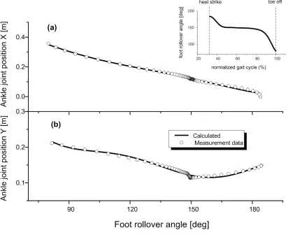
Kinematics

In this study, the stance foot was modelled as a rigid body with a curved surface

rolling on the ground without slipping (Figure 2), such that the foot kinematics during

the stance phase are described by

  

= = ∆

) (

) (

ft an

ft an

g y

f x

θ

θ

(1)

where ∆x_an =x_an −x_an( hs), where x is the current x coordinate of the ankle joint, and _an

) ( hs an

x is the x coordinate of the ankle joint at heel strike.

Equations (1) were determined using kinematic data captured in the gait laboratory

using a six camera Qualisys motion analysis system, where the ankle joint was

considered to be the mid-point between lateral and medial malleolus (Ren et al, 2005).

Figure 3 shows the output of the foot model when the roll over shape is described by a

best fit third order Fourier series. The relative timings of heel-strike and toe-off were

also based on measurement data.

       ⋅ + ⋅ = ⋅ + ⋅ = ft ft ft ft an ft ft ft ft an d dg d g d y d df d f d x

α

θ

ω

θ

α

θ

ω

θ

During walking there is at least one foot in contact with the ground throughout the

gait cycle. Thus, the positions of the other joint centres in the multi-segment model

were derived from the location of the stance ankle joint.

       ⋅ ⋅ + = ⋅ ⋅ + =

∑

∑

θ

θ

where m is the number of segments in the chain connecting the stance ankle joint to

the ith joint and I( j) is a sign function, which is equal to 1 when the segment

belongs to the stance limb, or equal to -1 if the segment is in the contralateral limb.

Differentiating Equation (3) twice, the accelerations of the joint centres are,

       ⋅ − ⋅ ⋅ ⋅ − = ⋅ + ⋅ ⋅ ⋅ − =

∑

∑

θ

α

θ

ω

θ

ω

θ

α

Thus, given the segment angles, Equations (1) to (4) were used to calculate the

accelerations of each body segment mass centre were derived using anthropometric

data.

Kinetics

The inverse dynamics method was employed to calculate joint kinetics and

mechanical energy expenditure during walking. Since, in predictive modelling, the

ground reactions are initially unknown, the inverse dynamics method must be based

only on segmental motions. This differs from the conventional implementation of

inverse dynamics used in gait laboratory studies (Winter, 1990; Siegler and Liu, 1997),

where the calculations start from the measured ground reactions.

The equations of motion of the ith body segment can be written as follows,

       + + = ⋅ ⋅ + + = ⋅

∑

∑

∑

α

(5a & b)

where the segment has n joints connecting it to other segments. _i

By combining the equations of motion of all body segments, the sums of the external

forces and moments can be derived. Since, during walking, the only external forces

and moments acting on the human body, other than gravity, are the ground reactions,

these expressions can be written as,

       − ⋅ = − ⋅ =

∑∑

∑

∑

∑

∑

α

where n is the number of body segments in the model.

Therefore, during the swing phase, the ground reaction force acting on the single

supporting foot can be obtained directly from Equation (6a). However, in double

support phase, the ground reaction forces and moment (COP) are indeterminate. In

order to solve this problem, the linear transfer assumptions shown in Figure 4, and

introduced in Ren et al, 2005, have been used to model the transfer of the ground

reactions from one foot to the other during the double support phase. As Figure 4

shows, these linear transfer assumptions are in good agreement with published ground

reaction measurements (Winter, 1990).

During gait simulation, firstly, the ground reaction forces on each foot are calculated

from Equation (6a) and the linear transfer relationships. Starting from the supporting

feet and working up, segment by segment, the resultant force at each joint is

calculated using Equation (5a). Then, the ground reaction moments on each foot are

obtained from Equation (6b) and the linear transfer relationship for the centres of

pressure. Starting from the feet and working up segment by segment again, the net

muscle moments at each joint are calculated using Equation (5b). A detailed

description of this inverse dynamics calculation process has been given elsewhere

(Ren et al, 2005).

Optimisation and the constraints associated with gait

It has been observed in experimental studies that people’s self-selected walking speed

Cavagna and Kaneko, 1977). Therefore, in this study, the optimisation problem was

described as: find segment trajectories that achieve the specified gait parameters,

whilst minimizing energy cost, and satisfying the constraints associated with a

walking gait.

The segment trajectories were represented by a set of Fourier series,

∑

=

⋅ ⋅ + ⋅ ⋅ +

= n

k

i k i

k i

i a a k t b k t

1

) ( )

( )

(

0 ( cos( ω ) sin( ω ))

θ (7)

where n is the order of the Fourier series and

ω

where T is the period of the gait cycle. One of the advantages of using a set of _c

Fourier series is that they provide a representation of the gait motions that is implicitly

cyclic, avoiding the need to introduce explicit constraints.

Power spectrum analysis of reflective marker data, during normal walking, has shown

that most of the signal power (99.7%) is contained in frequencies below 6Hz (Winter,

1990). Therefore, a set of 5th order Fourier series were employed to represent the

segmental rotations, resulting in a total of 11 Fourier coefficients for each segment,

which were used as the optimisation parameters.

In normal walking, bilateral symmetry can be assumed, that is, movements of the left

limb mirror movements of the right limb with a half cycle phase difference. Thus, the

number of DOF representing the 7-segment model is reduced to 4, resulting in 44

noted that doing this does not impose any symmetry constraint on trunk motion. In

fact, the optimiser can choose whichever pattern of trunk motion is most energy

efficient.

As suggested by experimental observations of walking energetics (Ralston, 1976;

Cavagna and Kaneke, 1977; Inman et al, 1994), a minimal energy criterion was

employed as the objective function. In particular, the total joint work over the gait

cycle was minimised.

Task constraints, biomechanical constraints and environmental constraints were

implemented in the optimisation scheme. The task constraints (input gait descriptors)

were average walking velocity V , cycle period _a T , and double stance duration. The _c

biomechanical constraints prevent joint hyperextensions or other unrealistic

movements. The environmental constraints represent the rules of ground interaction

during walking.

All of the above leads to the following mathematical definition of the optimisation

problem. Minimise mechanical energy expenditure over a complete gait cycle, which

is defined as follows,

∫ ∑

− ⋅ = Tc n

i

i d i p i

m T dt

E Minimise

0 1

) ( ) (

)

(ω ω

where T is the net muscle moment at the i_i th joint,

ω

velocities of the proximal and distal segments respectively. The optimisation

5th order Fourier series representing the rotations of trunk, thigh, shank and foot.

Furthermore, the optimisation is subject to the following constraints:

(1) Segment motion constraints:

] , 0 [ , ) (

0≤θi t ≤π t∈ Tc (i=1,2,3,4)

(2) Joint motion constraints:

] , 0 [ , ) ( ) ( , ) ( )

( _{3 max}(1) _min(2) _{4 3 max}(2)

2 ) 1 (

min ≤θ t −θ t ≤θ θ ≤θ t −θ t ≤θ t∈ Tc

θ

(3) Kinematic constraints:

0 ) (t >

ytip for a swing foot and ytip(t)=0 for a stance foot, where y is the vertical tip

position of the foot’s lowest point.

(4) Kinetic constraints:

0 ) (t >

F_y and _x

y x x t F t F

_µ

µ

−

) (

) (

for a stance foot, where µ_x is the friction coefficient

between the foot and the ground surface

(5) Stride length constraint:

c a an

c

an T x V T

x ( )− (0)= ⋅

For the purposes of calculating the energy cost from the inverse dynamics calculations,

200 discrete calculation points were used over the gait cycle. The constraints defined

above, and the representation of the segmental rotations by a set of finite Fourier

series, ensure that solutions for this optimisation problem are valid cyclic walking

gaits. However, this does not guarantee that they will be realistic.

The optimisation scheme was implemented in MATLAB using a Sequential Quadratic

Programming (SQP) algorithm (Gill et al., 1981) from the optimisation toolbox. The

c

T = 1.0 s and double stance duration = 0.18 s) were obtained from the gait

measurement data of one male subject (age: 38years, weight: 101.7kg, height: 178cm).

A detailed description of the experimental procedures has been given elsewhere (Ren

et al, 2005). The initial values of the optimisation parameters (Fourier coefficients)

were set such that the model stands upright and stationary. In other words, except for

the constant offset terms (a ), all of the Fourier coefficients were set to zero. In ₀(i)

order to avoid finding a single local minimum, different initial values were randomly

selected. These all represented stationary postures close to the upright position, as

these were found to have a very good chance of converging to a solution. Due to the

highly non-linear nature of the gait model, there appeared to be many local minima.

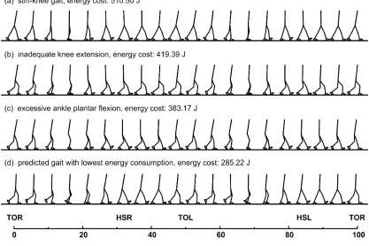
Results

Although many optimisation solutions were found, based on the major features of the

gait patterns, they appeared to fall into 4 distinct families of solutions, with only small

differences between members of the same family. We believe that these four families

represent just four local minima and that the small differences are related to the

precision of the optimisation process and the sensitivity of the objective function close

to the true minima. The four gait patterns (families) are illustrated in Figure 5. Each

family of gait patterns is represented by the member with the lowest energy cost. The

gait patterns in Figures 5(a), 5(b) and 5(c) differ from normal walking in certain

respects, which results in higher mechanical energy expenditure. The solution with

the lowest energy consumption (Figure 5(d)) also yields the most realistic gait pattern.

which provides further evidence that minimisation of energy consumption is a feature

of normal walking.

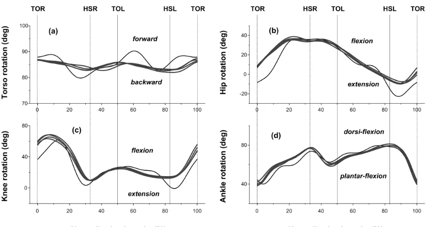
The predicted torso and lower limb joint rotations for the minimum energy solution

are depicted in Figure 6 and compared with gait measurement data. Over most of the

gait cycle, the majority of the predicted motions are in good agreement with the

measurement data. The largest differences occur in the trunk segment. Although the

overall trend agrees with the gait measurements and the reported data in the literature

(Inman et al., 1994), the amplitude of fluctuation is noticeably larger. This difference

could be due to the arms and pelvis not being considered, which probably moderate

the trunk’s angular fluctuations during normal walking. Another notable discrepancy

is thigh rotation, which is much lower than the measured data shortly after opposite

heel strike, thereby resulting in an increased range of thigh rotation. This is probably

because the model does not include pelvic transverse rotation, which increases stride

length, and the model compensates by increasing the thigh’s angular displacement to

achieve the specified stride length.

In Figure 7, the predicted ground reaction forces are compared with force plate data.

Although agreement is reasonable where trends are concerned, there are unexpected

fluctuations in the predicted forces. This probably arises from model simplifications,

for example, because rotations of the pelvis are neglected.

In this study, all segmental motions and ground reactions were predicted from only

three simple gait descriptors: average forward velocity, gait cycle period and double

stance duration, which minimizes the requirements for measurement data. No

prescribed motion patterns or measured trajectories were imposed on the model. This

is in contrast to previous work using a forward dynamics approach to gait prediction,

where the initial and final kinematic states where taken to be as measured and

imposed as optimisation constraints (Anderson and Pandy, 2001).

The predicted motions agree well with the measurement data over most of the gait

cycle. The agreement with measured ground reaction forces is reasonable, but there

are unexpected fluctuations. Moreover, among the local minima found, the solutions

with the lowest energy consumption produced the most realistic gait patterns. This

implies that minimizing energy cost is a primary motor control objective in normal

walking. This seems a reasonable inference for the lower limbs, since it has been

found that the cyclic movement of the legs accounts for the majority of the energy

cost of walking (Pierrynowski et al, 1980). This is supported by the fact that the

predicted motions of the lower limbs showed better agreement with the measured data

than those of the trunk segment.

The large predicted trunk motions are partly explained by the fact that the arms and

pelvis are not modelled. However, it has been shown in experimental studies that

head motion is smoother than that of the pelvis and the shoulder (Cappozzo et al.,

1978; Cappozzo, 1981), which may be due to the requirement to protect the visual and

vestibular systems from excessive mechanical disturbance. If so, minimisation of head

motions. This suggests that multiple performance objectives are employed in human

walking (Marshall et al, 1989).

The differences between the model predictions and experimental data are probably a

result of the limitations of the seven-segment model. Many of the discrepancies may

be due to the model being limited to the sagittal plane and the fact that the pelvis and

arms have been omitted. Pelvic transverse rotation increases stride length and

decreases the angular thigh excursion. Moreover, pelvic tilt can help to decrease and

smooth the trajectory of the body mass centre (Inman et al, 1994).

The use of inverse dynamics, instead of forward dynamics, has several advantages

including its computational efficiency, which is very important for predictive models

that are based on optimisation techniques. Since no numerical integration of the

differential equations is involved, the execution time for each optimisation iteration is

greatly reduced. For example, the prediction model proposed in this paper required

only 20 minutes of CPU time to converge to a minimal energy solution (Intel Pentium

4, 3.2 GHz). Another advantage of inverse dynamics is simpler implementation of the

kinematic and kinetic constraints associated with walking.

The authors plan to extend this work by creating a full three dimensional gait

prediction model. In addition, some of the variables that are currently fixed (gait cycle

duration, stride length etc) could be free to vary during optimisation, allowing further

Acknowledgements

Funding for this work has been provided by the UK Ministry of Defence. The

References

Anderson, F.C. and Pandy, M.G. (2001). Dynamic optimisation of human walking.

ASME Journal of Biomechanical Engineering 123, 381–390.

Cappozzo, A. (1981). Analysis of the linear displacement of the head and trunk during

walking at different speed. Journal of Biomechanics 14, 411–426.

Cappozzo, A., Figura, A., Leo, T. and Marchetti, M. (1978). Movements and

mechanical energy changes in the upper part of the human body during walking. In:

Asmussen, E. and Jorgensen, K. (eds.), Biomechanics VI-A. Baltimore, MD:

University Park Press.

Cavagna, G.A. and Kaneko, M. (1977). Mechanical work and efficiency in level

walking and running. Journal of Physiology 268, 467–481.

Channon, P.H., Hopkins, S.H. and Pham, D.T. (1992). Derivation of optimal walking

motions for a bipedal walking robot. Robotica 10, 165–172.

Chevallereau, C. and Aoustin, Y. (2001). Optimal reference trajectories for walking

and running of a biped robot. Robotica 19, 557–569.

Chow, C.K. and Jacobson, D.H. (1971). An optimal programming study of human gait. Mathematical Biosciences 10, 239–306.

Davy, D.T. and Audu, M.L. (1987). A dynamic optimisation technique for predicting

muscle forces in the swing phase of gait. Journal of Biomechanics 20, 187–201.

de Leva, P. (1996) Adjustments to Zatsiorsky-Seluyanov’s segment inertia parameters.

Journal of Biomechanics 29, 1223–1230.

Gill, P.E., Murray, W. and Wright M.H. (1981). Practical Optimization, Academic

Press, London.

Inman, V.T., Ralston, H.J. and Todd, F. (1994). Human locomotion. In: Rose, J. and

Koopman, B., Grootenboer, H.J. and de Jongh, H.J. (1995). An inverse dynamics

model for the analysis, reconstruction and prediction of bipedal walking. Journal of

Biomechanics 28, 1369–1376.

Marshall, R.N., Wood, G.A. and Jennings, L.S. (1989). Performance objectives in

human movement: A review and application to the stance phase of normal walking.

Human Movement Science 8, 571–594.

McMahon, T.A. (1984). Muscles, Reflexes, and Locomotion. Princeton University

Press, Princeton, NJ.

Pandy, M. G. (2001). Computer modeling and simulation of human movement.

Annual Review of Biomedical Engineering 3, 245–273.

Pierrynowski, M.R., Winter D.A. and Norman R.W. (1980). Transfer of mechanical

energy within the total body and mechanical efficiency during treadmill walking.

Ergonomics 23, 147–156.

Ralston, H.J. (1976). Energetics of human walking. In: R.M. Herman et al., (Eds.).

Neural Control of Locomotion. Plenum Press, New York.

Ren L., Jones R. and Howard D. (2005). Dynamic analysis of load carriage

biomechanics during human level walking. Journal of Biomechanics 38(4), 853–863.

Siegler, S. and Liu, W. (1997). Inverse dynamics in human locomotion. In: Allard P.

et al. (Eds.), Three-dimensional Analysis of Human Locomotion. John Wiley and

Sons Ltd, Wiley, New York.

Winter, D. A. (1990). The Biomechanics and Motor Control of Human Movement

(2nd Edition). John Wiley and Sons Ltd, Wiley, New York.

Yamaguchi, G.T. (1990). Performing whole-body simulations of gait with 3-D,

Muscle Systems. Biomechanics and Movement Organization. Spring-Verlag, New

York.

Yen, V. and Nagurka, M.L. (1987). Suboptimal trajectory planning of a five-link

human locomotion model. In ASME Winter Annual Meeting, Biomechanics of

Normal and Prosthetic Gait, Boston, MA, USA.

Zajac, F.E. and Winters, J.M. (1990). Modeling musculoskeletal movement systems:

joint and body-segment dynamics, musculoskeletal actuation, and neuromuscular

control. In: Winters, J.M. and Woo, S.L-Y. (Eds.), Multiple Muscle Systems.

Biomechanics and Movement Organization. Spring-Verlag, New York.

Zajac, F.E., Neptune R.R. and Kautz, S.A. (2003a). Biomechanics and muscle

coordination of human walking. Part I: Introduction to concepts, power transfer,

dynamics and simulations. Gait and Posture 16, 215–232.

Zajac, F.E., Neptune R.R. and Kautz, S.A. (2003b). Biomechanics and muscle

coordination of human walking. Part II: Lessons from dynamical simulations and

Figures and Captions

Figure 1 The seven-segment model including 6 joints and the following segments:

the right and left thighs, shanks, and feet together with a HAT segment (head, arms

and trunk). Segmental angles

θ

θ

the global reference frame, counter-clockwise being positive. T₁, T₂, …, T are the ₆

Figure 2 The ankle-foot kinematic relationships during foot rollover in the stance

phase. The foot angular displacement is defined by the line connecting the ankle joint

centre and the 2nd metatarsal, and the x-axis. The displacement of the ankle joint along

Figure 3 Mathematical representation of ankle-foot kinematics during stance phase,

(a) x coordinate of ankle joint and (b) y coordinate of ankle joint, using 3rd order

Fourier series (black lines) compared with measurement data (circles). The subject

(age: 38years, weight: 101.7kg, height: 178cm) walked at 1.52 m/s, and the cycle

period was 0.98 s. Inset is the time trajectory of stance foot rotation angle in the

0.0 0.5 1.0

linear transfer linear transfer linear transfer

CoP_r + CoP_l

CoP_r

F_yr F_xr F_yl

F_xl F_yr + F_yl

F_yr

0.0 0.5

HCL TOR HCR TOL

TOR

Measurement Data

0.0 0.2 0.4 0.6 0.8 1.0

0.0 0.5 1.0

Walking Time ( s )

Figure 4 Calculated transfer ratios (solid line), based on linear assumptions,

compared with measurement data from Winter (1990). F , _xr F , _yr F and _xl F are the _yl

horizontal and vertical ground forces at the right and left foot. CoP_r and CoP are _l

centres of pressure for right and left foot. CoP is defined as ground reaction moment

about the ankle joint divided by vertical ground force M_z F_y. In the double support

phase from right heel contact (HCR) to left toe off (TOL), the vertical force transfer

ratio r_{t_fy} increases from 0 to 1, the horizontal force transfer ratio r_{t_fx} increases from

) (

_ HC

fx t

r to (_ ) TO

fx t

Figure 5 Some typical gait patterns (local minima) found during the random

optimisation runs. The model (weight 101.7 kg) walked at 1.50 m/s, with a cycle

period of 1.0 s. The right limb swing phase is from 0 to 32%, and the stance phase is

from 32% to 100%. The double support phase is from 32 to 50% and from 82 to

100%. (a) stiff-knee gait with limited knee flexion during swing phase, mechanical

energy expenditure 510.50J. (b) inadequate knee extension in stance phase, energy

cost 419.39J. (c) excessive ankle plantar flexion and consequently inadequate knee

extension at opposite heel strike, energy cost 383.17J. (d) gait pattern which best

Figure 6 Predicted rotations of the trunk (a), right hip (b), right knee (c) and right

ankle (d) in the sagittal plane (black lines), compared with measured data (grey lines)

from 4 repeated trials for one subject (age: 38years, weight: 101.7kg, height: 178cm).

The average walking speed was 1.50 m/s, and the average cycle period was 1.0 s. The

swing phase for the right limb is from 0 to 32%, and the stance phase is from 32% to

Figure 7 Predicted anterior-posterior ground reaction force (a) and vertical ground

reaction force (b) (black lines), compared with recorded force plate data (grey lines)

from 4 repeated trials for one subject (age: 38years, weight: 101.7kg, height: 178cm).

The average walking speed was 1.50 m/s, and the average cycle period was 1.0 s. The

swing phase for the right limb is from 0 to 32%, and the stance phase is from 32% to