Design and Comparison of Vector Quantization
Codebooks for Narrowband Speech Coding
Hiba Faraj
*, Selma Ozaydin
Department of Electronic and Communication Engineering, Cankaya University, Turkey
Copyright©2019 by authors, all rights reserved. Authors agree that this article remains permanently open access under the terms of the Creative Commons Attribution License 4.0 International License
Abstract Vector quantization codebook algorithms
are used for coding of narrow band speech signals. Multi-stage vector quantization and split vector quantization methods are two important techniques used for coding of narrowband speech signals and these methods are very popular due to the high bit rate minimization during coding of the signals. This paper presents performance measurements of multistage vector quantization and split vector quantization methods. We used line spectral frequencies for coding of the speech signals in codebook tables so as to ensure filter stability after quantization. The codebooks were generated by using the Linde-Buzo-Gray (LBG) algorithm. The tests were performed by selecting large amount of input data in training and test stages and to evaluate noise robustness of the methods, both noisy and clean speech signals were used. As a result, different codebooks were designed and tested in many stages and different bit rates to measure quantization performance. It is measured in terms of spectral distortion evaluation. We obtained the best result in 24bit multistage vector quantization codebook with a spectral distortion less than 1 dB for clean speech training data input. When we compared multistage and split vector quantization codebook spectral distortion results, multistage codebooks gave better performance in each option.Keywords Multistage Vector Quantization, Split
Vector Quantization, Linear Predictive Coding, Line Spectral Frequencies, Codebook Design1. Introduction
Coding algorithms minimize the bit rate of an input signal without any harmful loss in the signal quality. Digital coding of speech signals in narrowband coding is the process of obtaining a compressed representation of the input signals with a perceptual quality and for efficient transmission through a channel. While an uncompressed
stages in each bit rate. In this framework, we designed many MSVQ and SVQ codebooks and we compared their performances by measuring the SD results.
2. LBG Codebook Design Algorithm
The goal in designing an optimal vector quantizer is to obtain N-element reproduction vectors representing any input vector with minimum spectral distortion. The codebook is then designed and trained by the training input vectors. In training stage of vector quantization, speech signals are used for generation of codebooks. During training stage, LSF vectors are obtained from input speech signals. There is a well-known iterative algorithm, namely LBG algorithm [1], The LBG VQ design technique is an iterative K-means clustering algorithm. In LBG algorithm, L training vectors are clustered into M codebook vectors.
The LBG algorithm tends to require the initial codebook. At the beginning of the algorithm, there is an initial code vector which is set as an average for the entire training sequences. Then, the code vector is then split into two. Afterwards, these two coded vectors are split into four. The splitting process continues until the required amount of code vectors is attained. In encoding the real process, there is an input vector which searches for the best matching codebook from the obtained codebook. The function of the decoder is to work like a table look-up which receives the transmitted index and look at the codebook for the vector which corresponds to and then matched vector from the codebook is then used to represent the input vector.
The input to the LBG algorithm is a training speech sequence obtained from people of different groups and of different ages. The speech signals used in training stage must be free of background noise. The algorithm is formally implemented in Figure 1 and by the following recursive procedure:
Step 1:Design a 1-vector codebook, set m=1, Calculate centroid
𝐶𝑖 = 𝑇1∑𝑇𝑗=1𝑋𝑗 (1) 𝐶2𝑖−1= 𝐶𝑖 𝑋( 1 + 𝛿 ) (2) Where T is the total number of data vectors.
Step 2: Double the size of the codebook by splitting (divide each centroid 𝐶𝑖 into two close vectors)
𝐶2𝑖= 𝐶𝑖 𝑋( 1 − 𝛿 ) (3)
1≤ i≤ m, here δ is a small fixed perturbation scalar (let m = 2m) Set n = 0 here n is iterative time
Step 3: Nearest-Neighbor Search
Find the nearest neighbor to each data vector. Put 𝑋𝑗 in the partitioned set 𝑃𝑖 if 𝐶𝑖 is the nearest neighbor to𝑋𝑗
Step 4: Find Average Distortion.
After obtaining the partitioned sets P = (𝑃𝑖, 1≤ i ≤ m) set
n = n + 1, Calculate the overall average distortion
Figure1. Flow diagram of the LBG algorithm
𝐷𝑛= 1𝑇∑𝑖=1𝑚 ∑ (𝐷𝑗=1𝑇𝑖 𝑗(𝑖), 𝐶𝑖) (4)
Where 𝑃𝑖= { 𝑋1(𝑖), 𝑋2(𝑖), … … . . 𝑋𝑇
𝑖 (𝑖)}
Step 5: Centroid Update.
Find centroids of all disjoint partitioned sets 𝑃𝑖 by
𝐶𝑖= 1𝑇 ∑𝑇𝑖𝑗=1𝑋𝑗(𝑖) (5)
Step 6: Iteration 1.
If (𝐷𝑛−1− 𝐷𝑛) / 𝐷𝑛 > δ (6) go to step 3 otherwise go to step 7
Step 7: Iteration 2.
If m = N then take the codebook 𝐶𝑖 as the final codebook; otherwise, go to step 2. N is the codebook size.
3. Split Vector Quantization
consideration, and then they are separately quantized. Then, the quantization of the subvectors in the codebooks is performed in each stage. Training the codebooks for SVQ is straightforward because each codebooks in the stages can be treated like a separate conventional vector quantizer, and can thus be trained separately using the K-mean algorithm.
When designing SVQ codebooks in our algorithm, in order to find the optimal partitioning for the LSF vectors by dividing the vectors into sub stages. There are many techniques when designing the codebooks in the MSVQ. The simplest method is to train the codebooks sequentially. Here, the codebook for the first stage is computed by using K-mean algorithm and the training data is quantized with the obtained one-stage vector quantizer. The resulting quantization error vectors are used for the second stage. This is repeated for all stages, with each new codebook trained using the error between the original and the reconstructed vectors including all the previous stages. In a 3-stage vector quantization, the LPC parameter vector (in some suitable representation such as the LSF
representation) is quantized by the first-stage vector quantizer and the error vector e (which is the difference between the input and output vectors of the first stage) is quantized by the second-stage vector quantizer [6]. The final quantized version of the LPC vector is obtained by summing the outputs of the three stages.
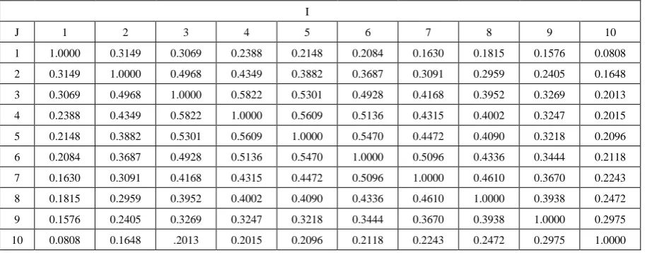
To minimize the complexity of the 3-stage vector quantizer, selection of a proper distortion measure is the most important issue in the design and operation of a vector quantizer. Since the spectral distortion is used here for evaluating LPC quantization performance, ideally it should be used to design the vector quantizer. However, it is very difficult to design a vector quantizer using this distortion measure. Therefore, simpler distance measures (such as the Euclidean and the weighted Euclidean distance measures) between the original and quantized LPC parameter vectors. The intra-frame correlation was calculated over the whole training database as a correlation between LSFi and LSFj in the same frame, i, j = 1,2,…,10. The intra-frame correlation coefficients are given in Table 1. The correlation between successive LSFs is significant [4].
Table 1. The intra-frame correlation coefficients
I
J 1 2 3 4 5 6 7 8 9 10
1 1.0000 0.3149 0.3069 0.2388 0.2148 0.2084 0.1630 0.1815 0.1576 0.0808
2 0.3149 1.0000 0.4968 0.4349 0.3882 0.3687 0.3091 0.2959 0.2405 0.1648
3 0.3069 0.4968 1.0000 0.5822 0.5301 0.4928 0.4168 0.3952 0.3269 0.2013
4 0.2388 0.4349 0.5822 1.0000 0.5609 0.5136 0.4315 0.4002 0.3247 0.2015
5 0.2148 0.3882 0.5301 0.5609 1.0000 0.5470 0.4472 0.4090 0.3218 0.2096
6 0.2084 0.3687 0.4928 0.5136 0.5470 1.0000 0.5096 0.4336 0.3444 0.2118
7 0.1630 0.3091 0.4168 0.4315 0.4472 0.5096 1.0000 0.4610 0.3670 0.2243
8 0.1815 0.2959 0.3952 0.4002 0.4090 0.4336 0.4610 1.0000 0.3938 0.2472
9 0.1576 0.2405 0.3269 0.3247 0.3218 0.3444 0.3670 0.3938 1.0000 0.2975
[image:3.595.71.529.365.544.2]4. Multistage Vector Quantization
The MSVQ reduces the complexity in a vector quantizer (in some suitable representation such as the LSF representation) are used to design the LPC vector quantizer.
To find the best LPC parametric representation for the Euclidean distance measure, the study of the 3-stage vector quantizer with the distance measure in the following three domains: the LSF domain, the arcsine reflection coefficient domain and the log-area ratio domain is done [7]. The 3-stage vector quantizer performs better with the LSF representation than with the other two representations. The Euclidean distance measure used for vector quantization in the preceding section provides equal weights to individual components of the LSF vector, which obviously are not proportional to their spectral sensitivities. Weighted Euclidean distance was proposed to measure the LSF domain, which tries to assign weights to individual LSFs according to their spectral sensitivities. The weighted Euclidean distance measure between the test LSF vector f
and the reference LSF vector 𝑓^ is given by:
(6)
Where 𝒇𝒊 and 𝒇𝒊^are the i-th LSFs in the test and reference vector, respectively, and 𝑪𝒊 and 𝑾𝒊are the weights assigned to the i-th LSF. These are given by
(7) Where P(f) is the LPC power spectrum associated with the test vector as a function of frequency f and r is an empirical constant that controls the relative weights given to different LSFs and is determined experimentally. The three multi-stage vector quantizer block diagram is shown in Figure 2. In Multistage Vector Quantization the input vector s to be quantized is passed through the first stage of the vector quantizer so as to obtain the quantized version of the input vector 𝒔𝟏^ The quantization error or residual error
𝒆𝟏 = s - 𝒔𝟏^ at the first stage is the difference of the input vector and the quantized version of the input vector. The quantization error at the first stage is given as an input to the second stage vector quantizer to obtain the quantized version of the error vector 𝒆𝒊^ at the first stage. The quantization error at the second stage 𝒆𝟐 = 𝒆𝟏 - 𝒆𝟏^ is given as input to the third stage vector quantizer to obtain the quantized version of the error vector at the second stage
𝒆𝟐^ and this process continues for the required number of
stages. Finally the decoder takes the indices 𝑰𝒊 from each quantizer stage and adds the corresponding codewords to obtain the quantized version of the input vector 𝒔^ = 𝒔𝟏^ +
𝒆𝟏^ + 𝒆𝟐^
𝒆𝟏 = s - 𝒔𝟏^ (8)
𝒆𝟐 = 𝒆𝟏 - 𝒆𝟏^ (9)
𝒔^ = 𝒔𝟏^ + 𝒆𝟏^ + 𝒆𝟐^ (10)
Figure2. Codebook generation for different stages of MSVQ
10
2 i i i i=1
i
ˆ
)=
[C W (f -f )]
ˆ
d(f,f
∑
i r i
∑
∑
= − = −=
+
+
=
p k k k p k kk
z
A
z
a
z
a
z
A
1 1ˆ
1
)
(
ˆ
,
1
)
(
(11)2 1 2 / 2 2 / 2 10 0 1 1
0
(
)
)
(
ˆ
log
10
1
))
(
ˆ
),
(
(
∑
− =
−
≈
n nn j n N
N n j SD
e
A
e
A
n
n
z
A
z
A
d
π π (12)∑
==
T i N n jSD
e
dB
d
T
SDavg
1 2 / 2 2)
(
1
π (13)5. Spectral Distortion Calculation
To evaluate the performance of the MSVQ and SVQ codebooks, the spectral distortion (SD) was measured. Spectral distortion is one of the most frequently used objective measure technique for evaluating the performance of LSF quantizers. The quantization performance of LPC parameters can be evaluated by the average spectral distortion of all the frames. The spectral distortion of each frame is defined as the root mean squared error between the power spectral density estimate of the original and the reconstructed LPC parameter vector. The spectral distortion can be calculated by the following formula and defined in dB;
Where A(z) and 𝑨�(𝑧)denote the original and quantized pth order LPC polynomials, while 𝑛1 and 𝑛0 and correspond to lower (100Hz) and upper (3800Hz) frequencies respectively in our algorithm. A(z) is the optimal pth order linear predictor and 𝐴^(z) is the predictor with quantized coefficients. N = 256 point FFT is used. The SD value is calculated over the bandwidth of 0-4kHz due to the 8kHz sampled input speech data. The spectral distortion is evaluated for all frames in the test data and its average value is computed. This average value represents the distortion associated with a particular quantizer. As mentioned before, the average spectral distortion has been used extensively in the past to measure the performance of LPC parameter quantizers. Transparent coding means that the coded speech is indistinguishable from the original speech through listening tests. For a transparent coding of an LPC based quantization of speech, the average SD should be about approximately 1dB.
6. Design of SVQ and MSVQ
Codebooks and Performance
In this study, different codebooks were designed using K-mean algorithm. The multistage vector quantization and split vector quantization methods were used to generate the codebooks of bit rates from 14 to 24 bits/frames. Then, the
scheme is (3, 3, 4) in which the first split contains the first three components of the 10 dimensional LSF vector, LSF1−LSF3, the second split consist of LSF4−LSF6 while LSF7−LSF10 constitute the third split. For evaluating the performance of the 2-split VQ, the LSF vectors were split as (4, 6), (6, 4) and (5, 5). The quantizers were trained using K-mean algorithm and the maximum size of an individual codebook was restricted to 1024 vectors (10 bits) For 2-split quantizers. The spectral distortion results of 2-split & 3-split SVQ codebooks for clean speech input data can be seen in Table 2, 3 and 4, respectively. The spectral distortion results for noisy speech input data can be seen in Table 5 and Table 6.
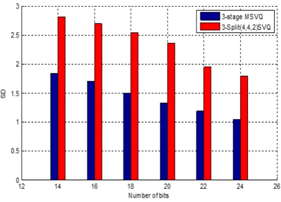
In split vector quantization we used two and three splitting’s. The results in Table 4 indicate that the best performance was obtained in (4,4,2) as shown in figure 3 split codebooks when we compared to (3,3,4) and (4,3,3). According to these results, we can say that when we use large codebooks for the first and second split, quantization accuracy increases according to other equal size codebooks. We can also say that, when we compare SD values of SVQ and MSVQ for the same bitrate codebooks, MSVQ gives better performance. Within 3-stage codebooks, we obtained best performance SD value in 24bit/frame.
Evaluation of the 3-split quantizers, relatively large codebooks can be used for the first and the second split. These codebooks should preferably be of equal sizes or alternatively one extra bit may be allocated for the second split. However, when the bit rate increases the largest allowed codebook size becomes as limiting factor and a few bits are wasted as they are forced to be allocated for the least significant third split. In our simulations, this limit was reached at the bit rate of 24, as the codebooks of the first two splits could not be enlarged and thus more than three bits had to be allocated for the last split. At higher bit rates, the best performance was obtained with the (4,4,2) splitting, where the largest codebook is required for the middle split and the codebooks for the first as well as for the third split can be of equal sizes or one extra bit can be allocated for the first split. Among the 2-split quantizers included, the best performance was obtained using the quantizer with (6, 4) splitting as long as the difference between codebook sizes could be maintained large enough. In multistage vector quantization a training speech sequence is 1st used to generate the codebook. Speech signal is segmented (windowed) into successive short frames and each frame of speech is represented by a vector. Tables 4 and Table 6 show the spectral distortion (dB), at various bit rates for a 3-stage multistage vector quantizer and 4-stage multistage vector quantizer, as we can see from the tables that with 3-stage gives better performance than in 4-stages in terms of SD. As shown in Figure 4 we compared 4-stage multistage vector quantization with the best 3-split in split vector quantization (4,4,2) as we can see that 4-stage MSVQ gives very good performance in SD.
The bit allocations for SVQ and MSVQ that yielded the best performance at different bit rates are given in Tables below.
Table 2. 2-split (SVQ) using clean speech
Bits/frame SD(dB) for (6,4)
SD(dB) for (5,5)
SD(dB) for (4,6)
14 2.81 2.75 2.90
16 2.49 2.51 2.53
18 2.22 2.20 2.24
20 2.11 2.04 2.03
Table 3. 3-split (SVQ) using clean speech
Bits/frame SD(dB) for (3,3,4)
SD(dB) for (4,4,2)
SD(dB) for (4,3,3)
14 2.95 2.82 3.13
16 2.78 2.70 3.03
18 2.50 2.55 2.59
20 1.28 2.36 2.28
22 2.01 1.95 2.07
24 1.86 1.80 1.84
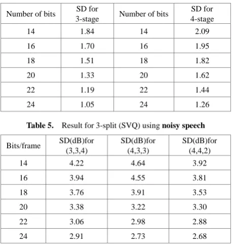
Table 4. Result for 3 and 4 stages (MSVQ) using clean speech
Number of bits SD for
3-stage Number of bits
SD for 4-stage
14 1.84 14 2.09
16 1.70 16 1.95
18 1.51 18 1.82
20 1.33 20 1.62
22 1.19 22 1.44
[image:6.595.306.538.135.361.2]24 1.05 24 1.26
Table 5. Result for 3-split (SVQ) using noisy speech
Bits/frame SD(dB)for (3,3,4)
SD(dB)for (4,3,3)
SD(dB)for (4,4,2)
14 4.22 4.64 3.92
16 3.94 4.55 3.81
18 3.76 3.91 3.53
20 3.38 3.22 3.30
22 3.06 2.98 2.88
24 2.91 2.73 2.68
Table 6. Result for 3 and 4 stages (MSVQ) using noisy speech
Number of bits SD for
3-stage Number of bits
SD for 4-stage
14 3.87 14 4.09
16 3.70 16 3.86
18 3.45 18 3.65
20 3.28 20 3.43
22 3.08 22 3.29
[image:6.595.307.537.367.616.2]Figure 3. 3-stage MSVQ and 3-split SVQ for clean speech
Figure 4. 4-stage MSVQ and 4-split SVQ for clean speech
7. Conclusions
The performance of two popular quantization methods, SVQ and MSVQ, was evaluated in LSF quantization. To achieve the best performance with MSVQ, it was found that the number of stages should generally be kept at minimum provided that maximum size codebooks are used for each stage. The evaluation of SVQ with 22 different splitting schemes indicated that none of the splitting schemes outperformed the others at all bit rates. In MSVQ two types of multistage were designed which are 3 and 4 MSVQ and calculating the spectral distortion for 33 different bit allocation. The bit allocation was more complicated with SVQ than with MSVQ because the optimal allocation depends on both the sub-vector lengths
and the frequency bands that the splits cover. The comparison between the quantization methods indicated that MSVQ clearly outperforms SVQ. By using MSVQ instead of SVQ, at least 2−3 bits can be saved without any quality degradations. In terms of SD as can been seen from tables and figures MSVQ gave better performance than SVQ.
REFERENCES
Y. Linde, A. Buzo, R.M. Gray, An algorithm for vector [1]
M.Suman, K.B.N.Prasanna ,Kumar, K.Kavindra Kumar , G. [2]
Phrudhi Teja “A new approach on Compression of Speech Signals using MSVQ and its Enhancement Using pectral Subtraction under Noise free and Noisy Environment”, Advances in Digital Multimedia 52 Vol. 1, No. 1, March 2012
P. Kroon and W. B. Kleijn. Linear Predictive Analysis by [3]
Synthesis Cod-ing, in Modern Methods of Speech Processing, Chapter 3. (Kluwer AcademicPublishers, 1995)
Ulpu Sinervo, Jani Nurminen, Ari Heikkinen, and Jukka [4]
Saarinen, “Evaluation of split and multistage techniques in22 LSF quantization”, 2003.
V. Krishnan, D.V. Anderson and K.K. Truong, “Optimal [5]
multistage vector quantization of LPC parameters over noisy channels”, IEEE Trans. Speech Audio Processing, Vol. 12, No. 1, pp. 1–8, Jan. 2004.
Kanawade. P. R, Gundal .S .S, “Tree structured vector [6]
quantization based technique for speech compression,” 237 International Conference on Data Management, Analytics and Innovation (ICDMAI), 2017.
Satya Sai Ram .M , Siddaiah .P, and M.Madhavi Latha, [7]
“Multi Switched Split vector quantizer,” International Journal of Computer, Information, and Systems Science, and Engineering, pp. 1-6, Winter 2008.
Kleijn. W. B, Paliwal .K.K, “An introduction to Speech [8]
coding,” Speech coding and synthesis, Elsevier science, pp.13 1-47, 1995.
Chin-Hui Lee, “Robust linear prediction for speech analysis,” [9]