An Iterative Method to Solve Nonlinear Equations

(1)

An Iterative Method to Solve Nonlinear Equations

Rubén Villafuerte1,*_{, Jesús Medina}1_{, Rubén A. Villafuerte S.}2_{, Victorino Juárez}1_{, Manuel González}3

1_{Faculty of Engineering, Universidad Veracruzana, México} 2_{National Institute of Technology, Campus Orizaba, México}

3_{Postgraduate in Biomedical Engineering Sciences, Universidad Popular Autónoma del Estado de Puebla (UPAEP), Puebla, México}

Abstract

In this paper, an iterative Newton-type method of three steps and fourth order is applied to solve the nonlinear equations that model the load flow in electric power systems. With the proposed method (N-1) non-linear equations are formulated and solved iteratively to calculate the Voltage in each node of an electrical system. The justification of the method and its theoretical preliminaries are presented in this paper. The proposed method is applied to IEEE test systems, and their results are compared obtaining a maximum error of 0.5%. From the results obtained, the proposed method is an alternative to solve load flows in electrical systems.

Keywords

Electric Power Systems, Iterative Methods, Load Flows, Non-linear Equations, Newton-Raphson

1. Introduction

There are different numerical methods for calculating the real roots of a nonlinear equation, and the most used is the Newton-Raphson method represented by equation (1) [1, 2].

xk+1= xk −_f′(xf(xk_k)₎ (1) Where:

f (xk): Nonlinear function evaluated in iteration k,

f '(xk): Derivative of non-linear function evaluated in

iteration k,

xk : Value of root in iteration k.

For solution of real nonlinear equations, several Newton-type methods have been proposed to reduce number iterations, increase the order of convergence and make a more efficient method [3,4,5,6]. The convergence analysis of equation (1) indicates that it has quadratic convergence and is represented by equation (2).

𝑒𝑘+1= 𝑓

′′_(𝛼)

2!𝑓′_(𝛼)𝑒𝑘2+ (𝑂)𝑒𝑘 3 (2) The Newton-Raphson method is widely used to calculate the roots of nonlinear equations where initial value xo so is sufficiently close to the root α and if the first

derivative of the function f(α) is non-singular. The efficiency of the Newton-Raphson method is 21/2_{, the base}

being the order of convergence and the denominator of the exponent, the number of evaluations; f (x) and f '(x). For solution of non-linear equations, multi-step methods with a higher order of convergence have been proposed, with the purpose of increasing the efficiency to more than 1.4142 [7-10]. In [10], the authors applied an iterative method of three steps and eighteenth order with an efficiency index of 1.513. In [11, 12], the authors propose methods of eighteenth order to reduce the number of iterations. In [13] the authors propose a two-step and sixth-order method with an efficiency of 1,431. In [14], the authors worked with a three-step method and fifteenth order of convergence which is represented by equation (3).

𝑦𝑘=𝑥𝑘−_𝑓𝑓_´((𝑥_𝑥𝑘) 𝑘)

𝑧𝑘=𝑦𝑘− �1− �𝑓(𝑦_𝑓(𝑥𝑘_𝑘₎)� 2

�𝑓(𝑦𝑘)

𝑓´(𝑦𝑘) (3)

𝑥𝑘+1=𝑧𝑘−_𝑓𝑓_´((𝑧_𝑧𝑘) 𝑘)−

𝑓 �𝑧𝑘− 𝑓_𝑓_´((𝑧_𝑧𝑘) 𝑘)� 𝑓´(𝑧𝑘)

Thus, different authors have proposed high-order, multi-step methods to solve a real nonlinear equation, all with the aim of increasing efficiency [15-20].

2. The Method and Analysis of

Convergence

In this section, the iterative method of three steps of the fourth order of convergence is constructed, for which the following basic definitions are necessary:

Definition 2.1. Let f Rm_{(D) be a function defined on an}

open interval D, and let α there be a simple zero of the nonlinear equation f(x) =0 and f’(α)≠0. An iterative method is said to have an integer order of convergence m if it produces the sequence {xn} of real numbers such that:

lim

𝑛→∞

𝑥𝑛+1− α

(𝑥𝑛− α)𝑚=𝐴 ≠0

(2)

or equivalently

𝑥𝑛−α= A(xn− α)m+ O((xn− α)m+1)

Definition 2.2. The efficiency of a method is measured by the index EI=ρ1/β_{, where ρ is the order of the iterative method}

and β is the total number of function evaluations per iteration. Now, we consider the iteration scheme:

yn=𝑥𝑛− �_𝑓´(𝑥𝑓(𝑥𝑛_𝑛)₎� 𝛼1 (4)

𝑧𝑛=𝑦𝑛− �_𝑓´(𝑥𝑓(𝑦𝑛_𝑛)₎� 𝛼2 (5)

𝑥𝑛+1=𝑧𝑛− �2𝑓(𝑦_(𝑓´(𝑥𝑛)𝑓(𝑥_𝑛₎₎2𝑛)� 𝛼3 (6) Where: α1, α2 and α3 are real constants

Theorem 2.1. Let α be a simple zero of sufficiently differentiable function f:D R → R for an open interval D. If xo is

sufficiently close to α, the method defined by equations (4), (5) and (6) has local order of convergence at least 4 with the following error equation

𝑒𝑛+1=𝑒𝑛4(10𝐶22+ 7𝐶2𝐶3−7𝐶23−4𝐶3) +𝑂(𝑒𝑛5) Where: 𝐶𝑘 = 𝑓

𝑘₍_α₎

𝑘!𝑓´(α);𝑘= 1,2,3.. and the error function is expressed as: en = xn- α Proof. Let α be a simple zero of f(x).

To carry out the convergence analysis of a numerical method, it is necessary to develop the function f (xn) and its

derivatives in Taylor series. Applying Derive program, we have the equation (7).

𝑓(𝑥𝑛) =𝑓′(𝛼 )(𝑒𝑛+𝐶2𝑒𝑛2+𝐶3𝑒𝑛3+𝐶4𝑒𝑛4+𝐶5𝑒𝑛5+𝐶6𝑒𝑛6) +𝑂(𝑒𝑛7) (7) The derivatives of the function f (xn), are also important for development in Taylor series of functions contained in any

numerical method. For step 1, the derivatives of the function f (xn) are represented by equations (8), (9), (10) and (11).

𝑓′(𝑥𝑛) =𝑓′(α )(1 + 2𝐶2𝑒𝑛+ 3𝐶3𝑒𝑛2+ 4𝐶4𝑒𝑛3+ 5𝐶5𝑒𝑛4+ 6𝐶6𝑒𝑛5) +𝑂(𝑒𝑛6) (8) 𝑓′′(𝑥𝑛) =𝑓′(α )(2𝐶2+ 6𝐶3𝑒𝑛+ 12𝐶4𝑒𝑛2+ 20𝐶5𝑒𝑛3+ 30𝐶6𝑒𝑛4) +𝑂(𝑒𝑛5) (9) 𝑓′′′(𝑥𝑛) =𝑓′(α )(6𝐶3+ 24𝐶4𝑒𝑛+ 60𝐶5𝑒𝑛2+ 120𝐶6𝑒𝑛3) +𝑂(𝑒𝑛4) (10)

𝑓𝑖𝑣₍_𝑥

𝑛) =𝑓′(α )(24𝐶4+ 120𝐶5𝑒𝑛+ 360𝐶6𝑒𝑛2) +𝑂(𝑒𝑛3) (11) With equations (7) and (8), we have equation (12).

𝑓(𝑥𝑛)

𝑓′_(𝑥_𝑛₎= en−C2en2+ (2C3−2C22)en3+ en4(4C23−7C2C3+ 3C4) + O(en5) (12)

Equation (4) and (12) give

𝑦𝑛=𝐶2𝑒𝑛2+ (2𝐶3−2𝐶22)𝑒𝑛3+𝑒𝑛4(4𝐶23−7𝐶2𝐶3+ 3𝐶4) +𝑂(𝑒𝑛5) (13) If it is defined:

𝑑𝑛=−_𝑓𝑓(𝑥′_(𝑥𝑛_𝑛)₎=−(𝑒𝑛− 𝐶2𝑒𝑛2+ (2𝐶3−2𝐶22)𝑒𝑛3+𝑒𝑛4(4𝐶23−7𝐶2𝐶3+ 3𝐶4) +𝑂(𝑒𝑛5) (14)

For step two, it is necessary to know the function f(yn). To do this, the development in Taylor series is done in the

neighborhood of the function f(yn), for which the equation (14) is important because it represents an approximation to the

zero of the function. Then, developing in Taylor series f(yn), in the neighborhood of dn, we have equation (15).

𝑓(𝑦𝑛) =𝑓 �𝑥𝑛−_𝑓𝑓(𝑥′_(𝑥𝑛_𝑛)₎�=𝑓(𝑥𝑛) +𝑓′(𝑥𝑛)𝑑𝑛+

1

2𝑓′′(𝑥𝑛)𝑑𝑛2+ 1

3!𝑓′′′(𝑥𝑛)𝑑𝑛3+ 1

4!𝑓(𝑖𝑣)(𝑥𝑛)𝑑𝑛4+𝑂(𝑑𝑛5) (15) Developing equation (15) in Taylor series with Derive, we have equation (16).

𝑓(𝑦𝑛) =𝑓 �𝑥𝑛−_𝑓𝑓(𝑥′_(𝑥𝑛_𝑛)₎�=𝐶2𝑒𝑛2+ 2𝑒𝑛3(𝐶3− 𝐶22)− 𝑒𝑛4(3𝐶23−7𝐶2𝐶3+ 4𝐶4) +𝑂(𝑒𝑛5) (16) From equation (16), until the third derivative equations (17), (18) and (19) are obtained.

𝑓`′(𝑦𝑛) =𝑓′(α )(2𝐶2𝑒𝑛+ 6𝑒𝑛2(𝐶3− 𝐶22)−4𝑒𝑛3(3𝐶23−7𝐶2𝐶3+ 4𝐶4) +𝑂(𝑒𝑛4) (17) 𝑓′′(𝑦𝑛) =𝑓′(α )(2𝐶2+ 12𝑒𝑛(𝐶3− 𝐶22)−12𝑒𝑛2(3𝐶23−7𝐶2𝐶3+ 4𝐶4) +𝑂(𝑒𝑛3) (18)

𝑓´´′(𝑦𝑛) =𝑓′(𝛿α )(12(𝐶3− 𝐶22)−24𝑒𝑛(3𝐶23−7𝐶2𝐶3+ 4𝐶4) +𝑂(𝑒𝑛2) (19)

(3)

From equation (8) and (16), with α2 = 1, we have equation (20).

�f(yn)

f´(xn)�=𝐶2𝑒𝑛

2_{+ 2}_𝑒

𝑛3(𝐶3− 𝐶22) +𝑒𝑛4(4𝐶23−7𝐶2𝐶3+ 3𝐶4) +𝑂(𝑒𝑛5) (20) If it is defined:

tn=−(𝐶2𝑒𝑛2+ 2𝑒𝑛3(𝐶3− 𝐶22) +𝑒𝑛4(4𝐶23−7𝐶2𝐶3+ 3𝐶4) +𝑂(𝑒𝑛5) (21) Developing f(zn) in Taylor series in the neighborhood of tn similar to (15), we have equation (22).

𝑓(𝑧𝑛) =𝑓 �𝑦𝑛−_𝑓𝑓(𝑦′_(𝑥𝑛_𝑛)₎�=𝐶2𝑒𝑛2+ 2𝑒𝑛3(𝐶3−2𝐶22)− 𝑒𝑛4(20𝐶23−17𝐶2𝐶3+ 2𝐶4) +𝑂(𝑒𝑛5) (22)

Substituting (13) and (20) in (5), we find zn

𝑧𝑛= 2𝐶22𝑒𝑛3− 𝑒𝑛4(9𝐶23−7𝐶2𝐶3− 𝐶4) +𝑂(𝑒𝑛5) (23) Developing the second term of (6) in Taylor series, we obtain equation (24), with α3 = 1.

�2f(yn)f(xn)

(f´(xn))2�= 2𝐶2

2_𝑒

𝑛3+ 2𝑒𝑛4(2𝐶3−5𝐶22) + 2𝑒𝑛5(19𝐶23−18𝐶2𝐶3+ 2𝐶4) +𝑂(𝑒𝑛6) (24) Substituting (23) and (24) in (6) and simplifying , we have the equation (25)

𝑥𝑛+1=𝑒𝑛4(−7𝐶23+ 10𝐶22+ 7𝐶2𝐶3−4𝐶3) +𝑒𝑛5(15𝐶24−19𝐶23−27𝐶22𝐶3+ 9𝐶2(2𝐶3+𝐶4) + 3𝐶32− 𝐶4) +𝑂(𝑒𝑛6) (25) Then, the three-step iterative method represented by (4), (5) and (6), is the fourth order of convergence and an efficiency index EI = 1.5874, only needs the evaluation of functions: f(xn), f´(xn) and f(yn)

3. Application in Electrical Power

Systems

In electrical engineering different studies are carried out in steady state, among them is the one known as; study of load flow. Network equations can be formulated systematically in a variety of forms. However, the node voltage method is the most suitable for power system analysis. The formulation of the network equations in the nodal admittance form results in complex linear simultaneous algebraic equations in terms of node currents. When node current are specified, the set of linear equations can be solved for the nodal Voltage. However, in a power system, powers are known than currents. Thus, the resulting equations in terms of power, known as the load flow equations, become nonlinear and must be solved by iterative techniques. Load flow studies, commonly referred to a load flow, are the backbone of power system analysis and design. They are necessary for planning, operation, economic scheduling and the exchange of power between utilities. In addition, load flow analysis is required for other analysis, such as transient stability and contingency studies. In solving a load flow problem, the system is assumed to be operating under balanced conditions and a single-phase model is used. Four quantities are associated with each node. These are: Voltage magnitude |V|, phase angle δ, real

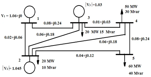
power P, and reactive power Q. The nodes are classified as: Slack node, Load nodes, and Regulated nodes. Figure 1 shows the single-line diagram of a five-node system [21]. Transmission lines are represented by their π equivalent, where impedances have been converted to per unit on a common MVA base.

(4)

[image:4.595.145.453.91.248.2]

Figure 1. Five node system For each node i of figure 1, we have an equation of the form (26).

𝑓𝑖(𝑉1,𝑉2, , ,𝑉𝑁) =𝑆𝑖∗− 𝑉𝑖∗�∑𝑁𝑗=1𝑌𝑖𝑗𝑉𝑗� i = 1, N-1 (26) Where:

N: Number nodes,

Si : Net complex power node i

Yij : Admittance between node i and node j,

Vi : Voltage node i,

Also: Yij, Vi, Si and fi(V1, V2, ... VN) are complex quantities and * means its conjugate of

The method consists of evaluating in each step equation (26) and its derivative with respect to the Voltage. Then, for each step, we have:

Step 1: Equation (4)

𝑉_𝑖𝑝1(𝑘+1)=𝑉_𝑖𝑝𝑜(𝑘)− � 𝑆𝑖∗−𝑉𝑖𝑝𝑜∗(𝑘)�∑𝑁𝑗=1𝑌𝑖𝑗𝑉𝑗𝑝𝑜(𝑘)�

𝜕 𝜕𝑉𝑖𝑝𝑜(𝑘)�𝑆𝑖

∗_−𝑉

𝑖𝑝𝑜∗(𝑘)�∑𝑁𝑗=1𝑌𝑖𝑗𝑉𝑗𝑝𝑜(𝑘)��

�𝑎1 i = 1, N, i ≠ slack (27)

𝑉_𝑖𝑝2(𝑘+1)=𝑉_𝑖𝑝1(𝑘+1)− � 𝑆𝑖∗−𝑉𝑖𝑝1∗(𝑘+1)�∑𝑁𝑗=1𝑌𝑖𝑗𝑉𝑗𝑝1(𝑘+1)�

∗_−𝑉

𝑖𝑝𝑜∗(𝑘)�∑𝑁𝑗=1𝑌𝑖𝑗𝑉𝑗𝑝𝑜(𝑘)��𝑎2 i = 1, N, i ≠ slack node

(28)

𝑉_𝑖𝑝3(𝑘+1)=𝑉_𝑖𝑝2(𝑘+1)− �2�𝑆𝑖∗−𝑉𝑖𝑝𝑜∗(𝑘)�∑𝑗=1𝑁 𝑌𝑖𝑗𝑉𝑗𝑝𝑜(𝑘)��𝑆𝑖∗−𝑉𝑖𝑝1∗(𝑘+1)�∑𝑁𝑗=1𝑌𝑖𝑗𝑉𝑗𝑝1(𝑘+1)��

∗_−𝑉

𝑖𝑝𝑜∗(𝑘)�∑𝑁𝑗=|𝑌𝑖𝑗𝑉𝑗𝑝𝑜(𝑘)��

2 �𝑎3 i = 1, N, i ≠ slack node (29)

4. Results

Applying the Law of Voltages to system of Figure 1, we have the non-linear equations (30), (31), (32) and (33).

(19.712⌊−71.51o_)V

1V2∗+ (34.177⌊−71.52o)V2V2∗+ (5.27⌊108.43)V3V2∗+ (5.27⌊108.43)V4V2∗+

(7.905⌊108.43)V5V2∗= 0.2 + 0.1i (30)

(3.952⌊108.43o_)V

1V3∗+ (5.27⌊103.43)V2V3∗+ (40.793⌊−71.54o)V3V3∗+ (31.622⌊108.43)V4V3∗= 0.1 + 0.15i (31)

(5.27⌊108.43o_)V

2V4∗+ (31.622⌊108.43)V3V4∗+ (40.793⌊−71.54o)V4V4∗+ (3.952⌊108.43)V5V4∗=−0.5 + 0.3i (32)

(5)

Three programs in FORTRAN were developed to solve the system represented in figure 1 and the test systems 30 and 118 nodes [31]. The first program (M1) corresponds to the eighteenth order iterative method [10]. The program (M2) corresponds to an iterative method of fourteenth order [32]. The program (M3) corresponds to proposed fourth order iterative method that has an efficiency of 1.5874. The equations (30),(31),(32) and (33) for the network of five nodes of Figure 1, or similar equations for larger systems are solved iteratively with three-step methods with different efficiency indices. In the solution of non-linear equations (30), (31), (32) and (33), there are restrictions that must be met in an iterative process, nodes two and three are P, V, therefore the voltage remains constant. The value of V1, is known, therefore, does not

enter to iterative process, which implies solving only (N-1) non-linear equations. The initial condition for voltages that have no restrictions is 1.0 + 0.0i [24,27,28]. The criterion to finish the iterative process is given by (34)

εt =�Vin+1−Vin

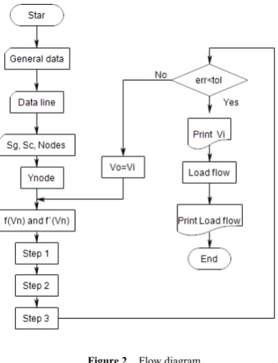
V_in � ≤tol i=1, N, i ≠ slack node (34) In Figure 2, a flow diagram is shown indicating the main points of the three-step method presented here. In the first block, general data are read, such as; the number of nodes, number of transmission lines, base power, slack node, tolerance and transformers. In second block data of transmission lines are read so that in the fourth block the admittance matrix Y is generated. In the third block, complex power generated and demanded in each node is read, to be used in block five for the formation of functions f (V) and its derivative. The generated functions are used in each step applying equations (27), (28) and (29) to calculate Voltages of the system under study. When completing the convergence, the iterative process ends.

Three cases are analyzed, and are described below

4.1. Case 1

For system of figure 1 with data shown, solve equations

[image:5.595.317.518.125.387.2]

(30),(31),(32) and (33) applying proposed methods in [10, 32] and M3 method, the values obtained are shown in table 1. The tolerance in each method was 0.001

Figure 2. Flow diagram

Table 1. Voltages obtained with methods M1, M2 and M3

Node M1(iter = 7) M2(iter = 11) M3(iter = 6)

|V| ∟Vo _|V| _∟Vo _|V| _∟Vo

1 1.0600 0 1.0600 0 1.0600 0

2 1.0450 -1.777 1.0450 -1.773 1.0450 -1.776

3 1.0300 -2.655 1.0300 -2.648 1.0300 -2.654

4 1.0186 -3.235 1.0186 -3.228 1.0186 -3.235

[image:5.595.305.536.412.517.2]

(6)

4.2. Case 2

In figure 3, a bar graph of voltages calculated with M1, M2, M3 and [31] is shown. In this case, factors α1 and α2 were

[image:6.595.124.480.137.296.2]

equal to 1.

[image:6.595.121.474.356.529.2]

Figure 3. Voltages obtained with (M1), (M2), (M3) and [31] Figure 4 shows the angle of the voltages of figure 3.

Figure 4. Angle Voltages figure 3

[image:6.595.132.472.578.733.2]

In figure 5, the value Voltages calculated with M1, M2, M3 and [31] is shown in a bar graph. In this case, the acceleration factors α1 and α2 for the M3 method were equal to 1.8 and 2.0, respectively

Figure 5. Voltages obtained with (M1), (M2), (M3) and [30] -20

-15 -10 -5 0

1 4 7 10 13 16 19 22 25 28

N

od

e an

gl

e (

de

g.)

Node number

M1 M2 M3 [31]

0.92 0.96 1 1.04 1.08 1.12

1 4 7 10 13 16 19 22 25 28

Nod

e V

ol

tage

(p

u.)

Node number

(7)

[image:7.595.113.485.104.283.2]

Figure 6 shows the angle of the Voltages of Figure 5.

Figure 6. Angle voltages for figure 4

[image:7.595.116.483.369.559.2]

4.3. Case 3

Figure 7 shows Voltages magnitude of 118 nodes. In the secondary axis the value reported in [31] is shown, in the primary axis values obtained with methods M1, M2 and M3.

Figure 7. System of 118 nodes, Voltages obtained with (M1), (M2), (M3) and [31]

Table 1 shows the results obtained from the five-node system and the errors observed are imperceptible. From point of view the number of iterations the M3 method seems to be best, however, execution time is of greater importance and in the three methods this was 15.6 milliseconds. In the system of 30 nodes, the maximum error found is 0.15%. This error can be related to tolerance used to finish iterative process. In Figure 6, corresponding to system of 118 nodes the maximum error oscillates around 0.5%. The simulation times are about 651.6, 806.8 and 140.4 milliseconds for method M1, M2 and M3, respectively. In the M3 method, values of α1 and α2 have an effect on execution time, and are selected by trial and error. The use of partial derivatives in the matrix formulation

generates a robust system that requires between 5 and 10 iterations when solving it, regardless of the size of the system. With the formulation used in this document, the number of iterations increases to 12 in the case of the system of 118 nodes when the appropriate values of the acceleration factors are selected with an execution time of 140.4 milliseconds, however, only equations (N -1) are solved and the formulation, as well as the solution is not very elaborate. Methods of eighteenth and fourteenth order that were adapted to compare their results with the M3 method, of figure 3, there is a lot of similarity, however for larger systems they have a longer execution time, or simply, they do not converge

-20 -15 -10 -5 0

1 4 7 10 13 16 19 22 25 28

An

gle

Vol

tage

(d

eg.)

Node number

M1 M2 M3 [31]

0.85 0.9 0.95 1 1.05 1.1

1 11 21 31 41 51 61 71 81 91 101 111

Nod

e V

olt

age

(p

u.)

Nod

e V

olt

age

(p

u.)

Node number

(8)

5. Discussion

One iterative method to calculate complex roots of a non-linear equation have been used in this work. The non-linear equation (26) is generated for each node of electric power system, with its first derivative with respect to the Voltages it is used for method proposed in this paper. One advantage of the proposed method is that they are simple to program and can be applied to large systems without need to apply special methods of solution, likewise, only (N-1) nonlinear equations are needed to find the solution. A disadvantage that can be associated with the technique applied to this work is a high iterations number, however, the use of multistep methods with acceleration factors is an option to reduce the execution time.

6. Conclusions

From the results obtained by application of the proposed method to solve test electrical power systems, the following concluding remarks can be written: 1) Only (N-1) non-linear equations are necessary; 2) Only f(xn), f'(xn) and

f(yn) are necessary to establish the method with an

efficiency index of 1.5874; 3) The results obtained are approximate, however, they are corrected, applying acceleration factors α1 and α2, reducing the number of

iterations and execution time; 4) Only the partial derivative of the Voltage is used in each iteration; 5) Formation of the jacobian matrix is not necessary; and 6) The results obtained are comparable with those reported in the specialized literature, there are differences that oscillate around 0.5%.

REFERENCES

[1] Nakamura S., Métodos Aplicados con Software, Prentice Hall Hispanoamericana de México, 1992

[2] Chapra Steven C. and Canale Raymond P., Numerical Methods for Engineers, McGraw-Hill Higher Education, 2014

[3] Homeier H.H.H, On Newton-Type Methods With Cubic Convergence, Journal of Computational and Applied Mathematics 205 1-5, 2005

[4] Kou Jisheng, Li Yitian, Wang Xiuhua, Third-Or Modification of Newton´s Method, Journal of Computational and Applied Mathematics 205, 1-5, 2007 [5] Petko D. Proinov and Stoil I. Ivanov, On the Convergence of

Halley’s Method for Multiple Polynomial Zeros, doi: 10.1007/s00009-014- 0400-7, Springer Basel , 2014 [6] Hueso José, Eulalia Martínez, Carles Teruel, Determination

of Multiple Roots of Nonlinear Equations and Applications, doi:10.1007/s10910-014- 0460-8, J Math Chem, 53:880– 892, 2015

[7] Xilan Liu, Xiaorui Wang , A Family of Methods for Solving Nonlinear Equations with Twelfth- Order Convergence, Applied Mathematics, 2013, 4, 326-329http://dx.doi.org/10 .4236/am.2013.42049 Published Online February 2013 (http://www.scirp.org/journal/am)

[8] Ramandeep Behl V. Kanwar, Highly efficient classes of Chebyshev-Halley type methods free from second-order derivative, Proceedings of 2014 RAECS UIET Panjab University Chandigarh, 06-08 March, 2014

[9] Sukhjit Singh and D. K. Gupta, A New Sixth Order Method for Nonlinear Equations in R, Hindawi Publishing Corporation the Scientific World Journal Volume 2014, Article ID 890138, 5 pages http://dx.doi.org/10.1155/2014/ 890138

[10]Mohamed S.M. Bahgat1, M.A. Hafiz, Three-Step Iterative Method With Eighteenth Order Convergence for Solving Nonlinear Equations, International Journal of Pure and Applied Mathematics Volume 93 No. 1 2014, 85-94, ISSN: 1311-8080 (printed version); ISSN: 1314-3395 (on-line version), url: http://www.ijpam.eu, doi:ttp://dx.doi.org/10.1 2732/ijpam.v93i1.7

[11]Nazir Ahmad and Naila Rafiq, Some Multistep Higher Order Methods for Nonlinear Equations, Academic Journals, Vol.9 (17). pp. 752-757, 15 September 2014, doi:10.5897/SRE20 14.5997,ISNN 1992-2248,http:/www.acacemicjournals.org/ SRE

[12]Bahgat Mohamed S.M and Hafiz M.A., Three-Step Iterative Method With Eighteenth Order Convergence for Solving Nonlinear Equations, doi: 10.12732/ijpam.v93i1.7, International Journal of Pure and Applied Mathematics, Volume 93 No. 1, 85-94, 2014

[13]Mohamed S. M. Bahgat, New Two-Step Iterative Methods for Solving Nonlinear Equations, Journal of Mathematics Research, Vol., 4, No 3, 2012

[14]A. Srivastava, An Iterative Method With Fifteenth-Order Convergence to Solve Systems of Nonlinear Equations, Computational Mathematics and Modeling, Vol. 27, No. 4, October, 2016, doi: 10.1007/s10598-016-9339-9

[15]Fazlollah Soleymany and S. Karimi Vanani, Numerical Solution of Nonlinear Equations by an Optimal Eigthth-Order Class of Iterative Methods, Ann Univ Ferrara (2013) 59:159-171, doi: 10.1007/s11565-012-0165-5 [16]Jovana Dzunic and Miodrag S. Petkovic, A Family of

Three-Point Methods of Ostrowski’s Type for Solving Nonlinear Equations, Hindawi Publishing Corporation Journal of Applied Mathematics Volume 2012, Article ID 425867, 9 pages doi:10.1155/2012/425867

[17]Ramandeep Behl V. Kanwar, Highly efficient classes of Chebyshev-Halley type methods free from second- order derivative, Proceedings of 2014 RAECS UIET Panjab University Chandigarh, 06-08, 2014

(9)

3204652, 6 pages, https://doi.org/10.1155/2017/3204652 [20]Alicia Cordero, Moin-ud-Din Junjua Juan R. Torregrosa,

Nusrat Yasmin, and Fiza Zafar, Efficient Four-Parametric With-and-Without-Memory Iterative Methods Possessing High Efficiency Indices, Mathematical Problems in Engineering Volume 2018, Article ID 8093673, 12 pages ttps://doi.org/10.1155/2018/8093673

[21]Hadi Saadat, Power System Analysis, third edition, PSA Publishing, 2010

[22]Tinney William. F., and Clifford E. Hart, Power Flow Solution by Newton's method, IEEE Transactions on Power Apparatus and Systems, vol. pas-86, no. 11, 1967

[23]Stott, B., and ALSAC, 0., Fast Decoupled Load Flow, IEEE, Trans., PAS-93, pp. 859-869 (1974)

[24]Stagg Glenn and Ahmed H. El-Abiad, Computer Methods in Power System Analysis, 270-276, McGraw Hill, 1968 [25]Tewarson R., Sparse Matrices, 72-75, Academic Press, New

York, NY, 1973

[26]Yaping Wang, Three-phase Power Flow Calculation of Low Voltage Distribution Network Considering Characteristics of Residents Load, IOP Conf. Ser.: Mater. Sci. Eng. 199 012061, doi:10.1088/1757- 899X/199/1/012061, 2017 [27]Hale H. V. and R. W. Goodrich, Digital Computation of

Power Flow-Some New Aspects, Trans. AIEE (Power Apparatus and Systems), vol. 78A, p. 919, 1959.

[28]Jizhong Zhu, Optimization of Power System Operation, Wiley and Sons, Inc, 2009

[29]ETAP software [30]EASYPOWER software

[31]http://www.ee.washington.edu/research/pstca/