International Journal of Emerging Technology and Advanced Engineering
Website: www.ijetae.com (ISSN 2250-2459, Volume 2, Issue 8, August 2012)95
Neural validation of FDBM Simulation for Formwork in
construction
Satya Prakash Mishra
1, Dr. D.K. Parbat
21 Associate Professor, Department of Civil Engineering, Bhilai Institute of Technology, Durg (C.G.) 2 Senior Faculty, Government Polytechnic, Sakoli, Maharashtra
Abstract— In spite of considerable development in
construction sector, the need of manual labour cannot be avoided. The India and other developing countries utilises intensive manual labour in building and infrastructures development. The methods used in these activities are either traditional or designed in a limited way. The present paper aimed to propose improvement in methods of performing these activities by developing mathematical simulation from data collected while the work was actually being executed in the field. Once the generalized model using all possible parameters developed, the weaknesses of the present method identified and improvement is possible. The main contribution of this paper is to develop the mathematical simulation of formworks placing sub activities in reinforced concrete construction and validate it with Neural Network prediction. Validation of the Field Data Based Mathematical(FDBM) model is achieved by comparing with the Artificial Neural Network Prediction and found satisfactory.
Keywords— FDBM simulation, Formwork, Reinforced
concrete construction, Reliability, sensitivity, ANN simulation.
I. INTRODUCTION
Construction activities (Gunnar Lucko et al., 2009) though appears simpler in execution but the relation between inputs and outputs shows a very complex pattern (H.Schenck, Jr, 1961). All framed structures constitutes Reinforced Concrete work (Suhad M. Abd et al. 2008; Kwangseog Ahn et al.2000) as a major activity and the cost of formwork(E. Sarah Slaughter et al.,1997) found to be 30-60 % of cost of framed structure.
This paper explains the mathematical simulation (Anu Maria 1997) of manual formwork fixing sub activity. The purpose of developing model was to overcome the deficiencies in current method, for process improvement, process management and to reduce fatigue in the workers and musculoskeletal injuries (John Rasmussen et al.2003; Kwangseog et al. 2000, Rwamamara et.al, 1988). The approach has been motivated from principles of construction management and Method study in industrial engineering (S. Dalelae 1991; K.H.F. Marrel 1967).
The work of this paper explained in following steps.
i. Formulation of FDBM model
(a) Study of the present method of manual Formwork fixing,
(b) Identification of Causes and Responses,
(c) Mathematical approach selected and development of model.
(d) Interpretation of model
ii. Results and analysis
iii. Validation of model using Neural Network
II. FORMULATION OF FDBMMODEL
a)Study of the present method of manual Formwork fixing:
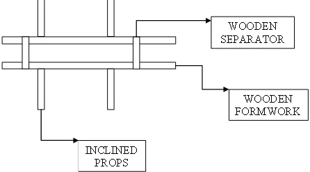
[image:1.612.332.555.505.629.2]Formworks are temporary structures, which are removed after concrete attains enough strength of a R.C.C. member. The formworks are built on site using timber planks and props for lateral supports at suitable intervals. The traditional timber formwork is preferred at common construction site and this is developed according to size and type of building components. Such as ground beam, beams supported from three sides, footings of columns, columns and slab forms.
Figure 1: Layout of work station of ground beam formwork
International Journal of Emerging Technology and Advanced Engineering
Website: www.ijetae.com (ISSN 2250-2459, Volume 2, Issue 8, August 2012)96 The two wooden frames kept vertically according to width of beam and they are kept apart by wooden separators and supported laterally with inclined wooden circular timber props.
b)Identification of Independent and Dependent variables:
Causes or dependent variables: The activity of formwork includes the workers data as input like anthropometric data, height, age and weight .The tools used in formwork are small hammer with one end as nail remover, Hacksaw for cutting timber planks and props there geometric dimensions are recorded as inputs as the each dimensions on varying influences the outputs. The workstation data such as size and nos. of planks and props with their dimensions and weight, size, diameter and nos. of nails required to fix a formwork and time required to complete a given size of form recorded.
The materials properties such as hardness in Rockwell hardness no. and shear strength of wood used .The environmental data such as ambient temperature, wind speed and humidity influences the output of workers so they are also recorded.
Dependent variables: For the formwork operations, the dependent variables would be:
(i) The extent of work done,
(ii) The human energy consumed and
(iii) The performance error in % of the required work.
[image:2.612.44.575.358.730.2]Extraneous Variables: These are other parameters, which could not identified, as inputs would be considered as extraneous variables such as loss of human energy by other means, effect of enthusiasm and motivations in workers performing the activity.
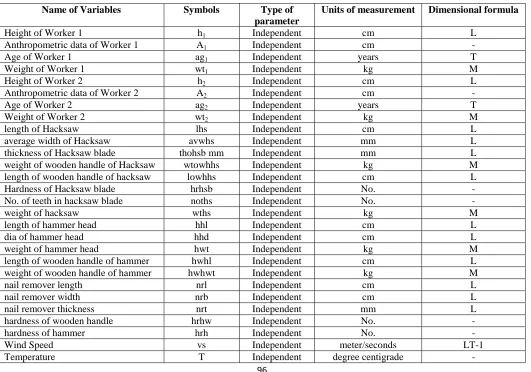
Table 1
Name of Variables, Symbols and Dimensional Equation of Variables
Name of Variables Symbols Type of
parameter
Units of measurement Dimensional formula
Height of Worker 1 h1 Independent cm L
Anthropometric data of Worker 1 A1 Independent cm -
Age of Worker 1 ag1 Independent years T
Weight of Worker 1 wt1 Independent kg M
Height of Worker 2 h2 Independent cm L
Anthropometric data of Worker 2 A2 Independent cm -
Age of Worker 2 ag2 Independent years T
Weight of Worker 2 wt2 Independent kg M
length of Hacksaw lhs Independent cm L
average width of Hacksaw avwhs Independent mm L
thickness of Hacksaw blade thohsb mm Independent mm L weight of wooden handle of Hacksaw wtowhhs Independent kg M length of wooden handle of hacksaw lowhhs Independent cm L
Hardness of Hacksaw blade hrhsb Independent No. -
No. of teeth in hacksaw blade noths Independent No. -
weight of hacksaw wths Independent kg M
length of hammer head hhl Independent cm L
dia of hammer head hhd Independent cm L
weight of hammer head hwt Independent kg M
length of wooden handle of hammer hwhl Independent cm L weight of wooden handle of hammer hwhwt Independent kg M
nail remover length nrl Independent cm L
nail remover width nrb Independent cm L
nail remover thickness nrt Independent mm L
hardness of wooden handle hrhw Independent No. -
hardness of hammer hrh Independent No. -
Wind Speed vs Independent meter/seconds LT-1
International Journal of Emerging Technology and Advanced Engineering
Website: www.ijetae.com (ISSN 2250-2459, Volume 2, Issue 8, August 2012)97
Name of Variables Symbols Type of
parameter
Units of measurement Dimensional formula
Humidity hu Independent %
Acceleration due to gravity g Independent m/sec 2 LT-2
length of wooden props lopp Independent meter L
Number of wooden props nopp Independent nos. -
Dia. of wooden props diaopp Independent meter L
weight of wooden props wtopp Independent kg M
hardness of wooden props hrppw Independent No. -
weight of wooden plank hrplw Independent No. -
Number of wooden plank nopl Independent no. -
length of wooden plank lopl Independent m L
width of wooden plank bopl Independent m L
thickness of wooden plank thopl Independent m L
weight of wooden plank wtpl Independent kg M
No. of nails non Independent nos. -
Hardness of nail hrn Independent No. -
diameter of nails don Independent m L
length of nails ln Independent m L
Initial Pulse Rate Of Worker1 Pi1 Dependent pulse/minute T -1 Final Pulse Rate Of Worker1 Pf1 Dependent pulse/minute T -1 Initial Pulse Rate Of Worker2 Pi2 Dependent pulse/minute T -1 Final Pulse Rate Of Worker2 Pf2 Dependent pulse/minute T -1
Duration t dependent minutes T
Extent Of Work done Af Dependent Meter2 L2
Actual area of formwork Afa Dependent Meter2 L2
c)Mathematical approach selected and development of model:
The mathematical relation between inputs and outputs could be of any form may be polynomial, exponential or log linear. The Buckingham theorem (S.P. Mishra et. al 2011 (2); Piotr D. Moncari et. al, 1981) found suitable for developing the model. As it states that if the inputs and outputs represented in dimensionless pie terms by dimensional analysis then they can be represented by eqn. (1).
a b c d e
Y k A B C D E …(1)
Moreover, the controls over the variables are not affected.
International Journal of Emerging Technology and Advanced Engineering
Website: www.ijetae.com (ISSN 2250-2459, Volume 2, Issue 8, August 2012)98
Pie terms:
Table 2
Combining of independent variables in Pie terms
Pie Terms Dimensionless equations
π1
2 2 2 2
1 1 1 1
A W Ag ht A W Ag ht
π2
hhl hhd hwhl wthh wtowh nrl nrt lhs avwhs lowhhs thob wths wtwh nrb
π3
60
vs Hu g t
π4
hrhsb hrh hrhw
hrn hrplw hrppw
π5 Noths
π6
lopp lopl lon thopl wtopp
dopp dopp bopl diaon wtpl
[image:4.612.37.572.392.562.2]
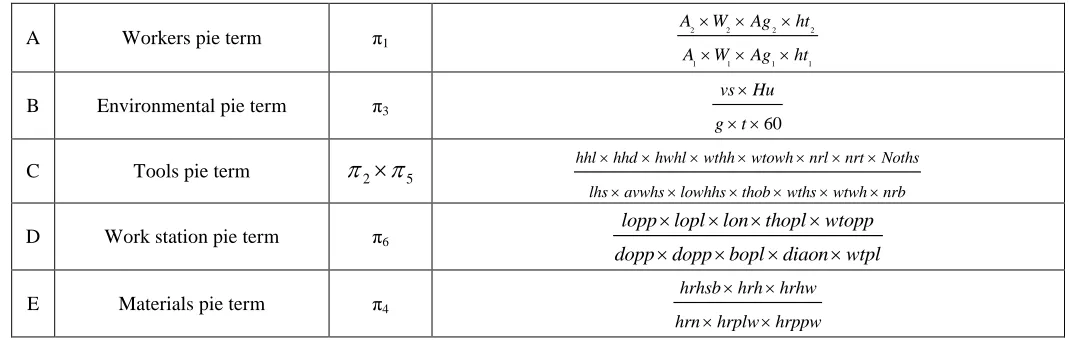
Table 3
Combining Independent Pie Terms: Above pie terms were further reduced in following A, B, C, D and E dimensionless pie terms–
A Workers pie term π1 2 2 2 2
1 1 1 1
A W Ag ht
A W Ag ht
B Environmental pie term π3
60
vs Hu g t
C Tools pie term
2
5 hhl hhd hwhl wthh wtowh nrl nrt Nothslhs avwhs lowhhs thob wths wtwh nrb
D Work station pie term π6 lopp lopl lon thopl wtopp
dopp dopp bopl diaon wtpl
E Materials pie term π4 hrhsb hrh hrhw
hrn hrplw hrppw
International Journal of Emerging Technology and Advanced Engineering
Website: www.ijetae.com (ISSN 2250-2459, Volume 2, Issue 8, August 2012)99 Table 4
Conversion of output data: Similarly the Dependent variables into Y1, Y2 and Y3 Pie Terms –
Extent of Work done Pie Term Y1
Af
lhs hhl
Human Energy Pie Term Y2
1 2 1 2
( ) ( )
2 2
Pf Pf Pi Pi
t
Performance Error (% Error in work done) Y3 100
Afa Af
Af
A, B, C, D, E are the final independent pie terms representing workers data, environmental data, tools data, workstation data and materials data and the response variable Y can be stated for all Y1, Y2 and Y3.
This dimensionless statement (1), transformed into linear relationship using log operation. The log linear relationship so obtained is easy to understand and does not damage any facets of original relationship.
For determining the indices of the relation between output and inputs, we use multiple regressions and Matlab software, thus the models for Y1, Y2 & Y3 obtained as under.
0.0259 1.0456 0.0815 0.4836 0.0047
1 1.057547 . . . .
Y A B C D E … (2)
0.0066 1.1617 0.3225 0.455 0.0017
2 1.000023 . . . .
Y A B C D E … (3)
0.436 0.1844 0.0394 0.383 0.0024
3 1.000011 . . . .
Y A B C D E … (4)
III. RESULTS AND ANALYSIS
Interpretation of models: The numeral multiple of the equations represents the extraneous variables of the models. The indices to A, B, C, D and E in the equations represents relative waitage to affect the output variables. They represents a group of input variables as listed in Table 3 workers data, environmental data, tools data and work station data respectively.
[image:5.612.304.569.157.439.2]Sensitivity analysis: When a model has multiple input parameters then it becomes important to know for a certain value of positive and negative variation which parameter is influencing maximum and output parameter is sensitive up to what extent. To check the sensitivity of each model the set of output and input parameters are selected in which has minimum error in from Y observed. Sensitivity of a model is the percentage influence on Y, by 10% positive or negative variations keeping the other variable to its minimum error set.
Figure 2: Influence of individual input variable in % of Y1
[image:5.612.334.554.524.669.2]Figure 2 shows the comparative degree of influence by input variables in percentage on Y1 (Extent of work done).The figure represents that environmental data(B) and work station data (D) has significant influence but B is most influencing but effect is inversely proportional to variations. Extent by which it influences Y1 i.e., productivity indicated by the graph.
International Journal of Emerging Technology and Advanced Engineering
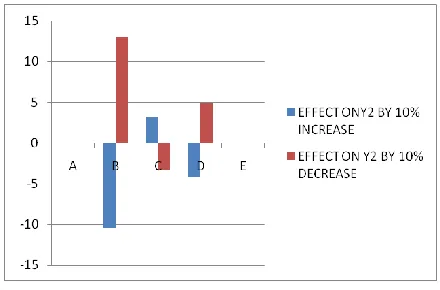
Website: www.ijetae.com (ISSN 2250-2459, Volume 2, Issue 8, August 2012)100 Figure 3 shows the influence of variations in inputs on Y2, which represents the Human energy consumption. The above figures imply that the input variable A is most influential and C is least influential. The A indicates the
ratio of workers data i.e., 2 1 W
W
and as A is influencing
[image:6.612.59.279.252.407.2]inversely, by positive increment in A the Y2 is reducing, so to reduce the Y2 worker 2 should be so selected that its anthropometric data be higher than worker 1.
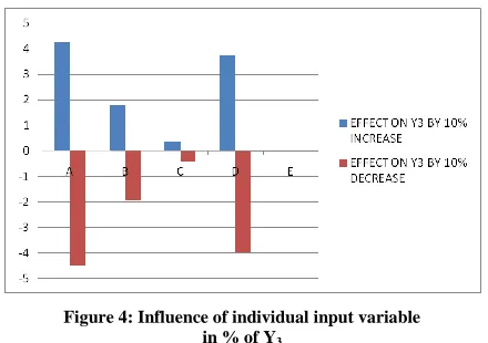
Figure 4: Influence of individual input variable in % of Y3
Figure 4 shows the degree of influence by individual input variables on Y3 Performance Error. The above figure clearly indicate that input variables A and D are highly influential to Y3, so to reduce the Y3 we should reduce A and D.
[image:6.612.100.238.596.672.2]Optimization of the models: Having known the form of mathematical model it is the need to optimize the models. Since in this study the no. of variables are more than one for optimization analysis using MS Excel Solver multivariate constrained optimization is performed. The MS Excel solver tools used generalized reduced gradient concept for optimization. Under the following constraints situation:
Table 5
Constraints for Multivariate optimization
Input terms max min
A 2.07 0.68 B 0.01 0.00 C 131.25 19.75 D 179.58 24.65 E 3.29 3.29
The Optimization results found are:
For Maximizing Y1 Extent of work done, the values of set of inputs A, B, C, D, and E in Eqn. (2) - 0.68, 0.01, 131.25, 24.65 and 3.29, provided maximum productivity pie term i.e., Y1 = 42.47.
For Minimizing Y2 i.e., Human energy, the set of inputs A, B, C, D, and E in Eqn. (3) should be 0.68, 0.01, 19.75, 179.58 and 3.29, provided minimum human energy Y2 = 50.60.
Similarly, for Minimizing Y3 Performance Error, the values of A, B, C, D, E in Eqn. (4) should be 0.68, 0.00, 19.75, 24.65 and 3.29, provided minimum performance error Y3 = 1.20.
IV. VALIDATION OF MODEL USING NEURAL NETWORK
Validation of FDBM models achieved by:
(i) Comparing the ANN simulation results with Field observed (Vahid K. Alilou, 2009; Tapir S.H. et Al, 2005).
(ii) By performing Reliability analysis of (S.P. Mishra et al., 2011-1)
ANN Simulation: ANN Simulation of the gathered field data using Matlab software have been performed. Which results into simulation based model and quantify appropriate non-linear behaviour of effect (responses) as influenced by causes (Inputs).
Reliability: Reliability of the individual model established using the following relation.
Reliability 1 Mean Error
( )
Mean Error
( )
i i
i
x f
f
Reliability 1 ( ) ( )
i i
i
x f
f
Where
xi is percentage error expressed in fraction and
fi frequency of occurrence
Mean error calculated by obtaining difference between observed values and respective values obtained from mathematical model with respect to observed value. Mathematically
Observed Value Mathematical Model Value Percentage Error
Observed Value
International Journal of Emerging Technology and Advanced Engineering
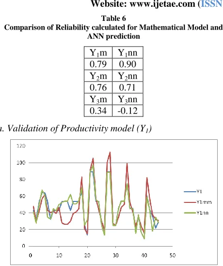
Website: www.ijetae.com (ISSN 2250-2459, Volume 2, Issue 8, August 2012) [image:7.612.51.281.121.395.2]101 Table 6
Comparison of Reliability calculated for Mathematical Model and ANN prediction
Y1m Y1nn 0.79 0.90 Y2m Y2nn 0.76 0.71 Y3m Y3nn 0.34 -0.12
[image:7.612.326.556.196.341.2]a. Validation of Productivity model (Y1)
Figure 5: Comparative plot of Y1, Y1cal and Y1nn (Neural Prediction)
[image:7.612.332.555.423.554.2]In Figure 5 on ordinates productivity in dimensionless pie terms and on abscissa the number of observations have been plotted which indicates the proximity and variations in observed output Y1, model output Y1cal with ANN predictions Y1nn thus validates the developed model for Extent of Work Done i.e., Productivity in Manual formwork Operation.
Figure 6: Comparative plot of Error in results of model and ANN prediction for Y1
Figure 6 compares the error in Y1 model results and errors in Y1nn simulation are distributed.
The reliability analysis of mathematical model and neural prediction for Y1 performed and found 0.79 and 0.90 respectively. Results indicate reliability of mathematical model is quite good and slightly less than neural prediction, thus validate the model.
b. Validation of Human Energy model (Y2)
Figure 7: Comparative Plot between observed Human energy (Y2),
model output (Y2m) and Neural Prediction (Y2nn)
The proximity of observed values of human energy Y2, calculated values from mathematical model Y2cal and neural network simulation results are plotted in Figure 7 which validates the mathematical model.
Figure 8: Comparative plot of errors by comparing field data with Y2model and Y2nn.
[image:7.612.57.281.499.642.2]International Journal of Emerging Technology and Advanced Engineering
Website: www.ijetae.com (ISSN 2250-2459, Volume 2, Issue 8, August 2012)102
[image:8.612.48.285.133.287.2]c. Validation of Performance Error Model
Figure 9: Comparative Plot between observed Human Energy (Y3),
Calculated (Y3mm) and Neural Network Prediction (Y3nn)
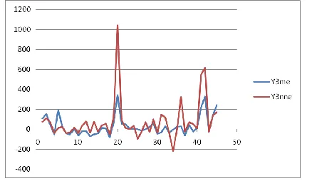
[image:8.612.61.280.390.517.2]The Figure 10 shows comparison between the actual fields recorded performance error Y3, Calculate value from model (4) Y3mm and Neural network prediction Y3nn. The graph indicates that Y3mm curve flatter than Y3nn and variations are small so the model Y3 considered as validated.
Fig. 10: Comparative plot of errors in values of performance error obtained by model Y3me and neural predictions, Y3nne
Figure 11 shows the percentage variations in calculated model results and neural network predictions from field observations Y3. Though some error are very high and Reliability of Y3m and Y3nn obtained 0.34 and -0.12 which may be very low as regard to Y3 but comparing the trend between Y3me and Y3nne, the mathematical model for performance error (4) is validated.
V. DISCUSSIONS
1. The mathematical models obtained from FDBM approach are in polynomial form and complex as each independent major pie terms are multiple of various input parameters as described in Table 3.
2. Interpretation of models gave extent of influence on output of the model by any pie terms or any variables listed in Table 1.
3. By comparing the indices of equation(1), as to maximize the productivity Y1 the absolute value of indices D found to be most influencing because it is highest whereas the negative sign indicates it should be minimized, further indices of E being positive and second highest it should be maximized. Thus, by analyzing the variables combined in developing D and E major pie terms one can easily suggest the method improvement to get required results.
4. Similarly in equation (2) Y2 human energy should be minimum, the indices of A, workers data being highest and with negative sign, it is found most influencing and needs to be minimized.
5. In equation (3), the indices of B environmental conditions at work place found to be most influencing and positive so to reduce the error in shearing of rebars minimized.
6. Sensitivity analysis suggest the degree of influence of variables A, B, C, D, E on output Y1,Y2,Y3. Desired values of the output obtained by adjusting inputs according to this analysis.
7. Optimization analysis suggests the optimum output achieved, if the results of this analysis incorporated in present method of Formwork fixing.
8. ANN simulation validates the model for Productivity, Human Energy and model of Performance Error. 9. Reliability of the FDBM model has been validated by
neural prediction.
10. Study of mathematical model output and developed ANN predictions for the phenomenon truly represents the degree of interaction of various independent variables.
VI. CONCLUSION AND SUGGESTIONS FOR FUTURE WORK
1. Field data based modelling concept thus found very useful and can be applied to any complex construction activity as the observations for variables are obtained directly from the work place and include all kind of data such as workers anthropometrics, environmental conditions, tools used and its geometry, layout of work station and materials properties.
International Journal of Emerging Technology and Advanced Engineering
Website: www.ijetae.com (ISSN 2250-2459, Volume 2, Issue 8, August 2012)103 3. Before finding the sensitivity of inputs, it is necessarily
to decide the validity of the models. This is so because though we have taken care to purify the observed data there is a chance of some impure data entering in the mathematical processing of the data.
4. The approach to decide the validity would be to substitute in the model known inputs for every observation & decide the difference in response by model and actually observed response. This will give us pattern of distribution of error & frequency of its occurrence.
5. The formulated models in this study are as per working conditions and environmental conditions of selected building construction sites. This needs to be tested for other working and environmental conditions.
6. It is suggested that the countries where the construction works involves intensive manual works, each activity should be analysed by making FDBM model and a new method of doing work can be developed in various types of construction.
7. The FDBM approach can be applied for Ergonomic construction, mechanization and prioritization in mechanization all kind of infrastructure construction as it has been seen that the non availability of construction workers leads to delay the major projects so ergonomic construction is the need of present scenario.
REFERENCES
[1] Anu Maria, (1997). Introduction to Modeling and Simulation. Proceedings of the 29th conference on winter simulation, 7-13. [2] Cheng-Jian Lin, (2007). Member, IEEE, and Jun-Guo Wang. Human
Body Posture Classification Using a Neural Fuzzy Network based on Improved Particle Swarm Optimization. ISIS 2007 Proceedings of the 8th Symposium on Advanced Intelligent Systems, 414-419. [3] Dalela, S. (1999). First edition, Text Book of Work Study and
Ergonomics. Standard Publishers Distributors, Nai Sadak, Delhi-6. [4] Tapir S.H. , J.M. Yatim and F. Usman, ―Evaluation of Building
Performance Using Artificial Neural Network: Study on Service Life Planning in Achieving Sustainability‖. The Eighth International Conference on the Application of Artificial Intelligence to Civil, Structural and Environmental Engineering, Rome, Italy. 30 August-2 Sept 2005.
[5] Marrel, K.H.F. (1967). McGraw Hill, Ist. Edision, The Man in his working Environment. Methods of investigating work and methods of measuring work and activity, 352-360, Practical Ergonomics.
[6] Modak, J.P. (2009). Application of AI (Artificial Intelligence) Techniques for Improvement of Quality of Performance of a Process Unit / Man Machine System: A Philosophy. Key- Note Lecture at A National Conference, Organised by Disha Institute of Technology and Management, Raipur, 14-16.
[7] Mishra, S.P., Parbat, D.K., and Modak, J.P. (2011). Literature Review on Field Data Based Mathematical Simulation of Complex Construction Activities. NICMAR, Journal of Construction Management (International), ISSN No. 0970-3675, XXVI (1): 78-88.
[8] Mishra, S.P., Modak, J.P., and Parbat, D.K., (2011). An Approach to Simulation of a complex Field Activity by a Mathematical Model. Industrial Engineering Journal (India), ISSN No. 0970-2555, II (20): 11-15.
[9] Mishra, S.P., Parbat, D.K., and Modak, J.P. (2011). Field Data Based Mathematical Simulation and Optimization of Complex Construction Activity. Invited by Project and Construction Managing Committee, Presented and Published in Proceedings of Association of Iron & Steel Technology Conference 2-5 May 2011, Indianapolis, Indiana, USA.
[10]Rwamamara Romuald and Holzmann Peter 2007 , ―Reducing the Human Cost In Construction Through Designing For Health And Safety – Development Of A Conceptual Participatory Design Model‖ Ph.D. Theses, Second International Conference World of Construction Project Management TU Delft, the Netherlands. [11]Piotr D.Moncari et al. (1981), A report on research project
Sponsored by the National Science Foundation, Department of Civil Engineering, Stanford University, California.
[12]Vahid. K. Alilou, Mohammad, ―Prediction of 28-day compressive strength of concrete on the third day using Artificial Neural Networks‖. Teshnehlab International Journal of Engineering (IJE), Volume (3): Issue (6), pp.565-576, 2009.
[13]Flood, I., Christophilos, P. (1996). Modeling construction processes using artificial neural networks. Automation in Construction, 4 (4): 307-320.
[14]Kwangseog, Ahn, Victor, L. Paquet, (2000). Ergonomic assessment of the concrete pouring operation during highway construction State University of New York at Buffalo.
[15]Fangyi, Zhou, Simaan, M. AbouRizk, Fernando, (2008). A Simulation Template for Modeling Tunnel Shaft Construction. Proceedings of the Winter Simulation Conference, 2455-2461. [16]Sanford, W. (1985). Sanford, W. (1985). Applied Linear Regression.
2nd Edition. Hoboken, NJ: John Wiley & Sons.