Thermal Conditions Controlled by Thermostats: An Occupational Comfort and Well being Perspective

(1)

Thermal Conditions Controlled by Thermostats: An

Occupational Comfort and Well-being Perspective

Qiuhua Duan

1

_{, Julian Wang}

1,2,*

1_{Department of Civil and Architectural Engineering and Construction Management, University of Cincinnati, USA} 2_{School of Architecture and Interior Design, University of Cincinnati, USA}

Abstract

From the perspective of occupational comfort and well-being, indoor thermal condition characterized by its temperature levels, spatial variations, and airflow patterns plays an important role. Studies have demonstrated strong correlations among indoor comfort levels and users’ well-being, productivity, and overall health. Computational fluid dynamics (CFD) has been used to investigate indoor thermal comfort. In this research, a private office on the University of Cincinnati campus was selected and studied in order to spatially map the thermal comfort index. Autodesk® CFD, a ventilation simulation software, was utilized to model the office space and air conditioning systems, as well as simulate the airflow in the indoor space. Based on the simulation results, the air speed, ambient temperature, and relative humidity were all obtained for different vent locations. These simulated parameters can be used in dynamic anthropometry to acquire the predicted mean vote (PMV) and temperature in specific office areas. Through this method, a visualized indoor comfort map was developed as a means of indicating potential user comfort effects; spatial variations in the indoor comfort index have also been analyzed and discussed.

Keywords

Occupational Comfort, Indoor Thermal Condition, Simulation, Offices

1. Introduction

Achieving a desirable indoor thermal environment is one of the major concerns in architectural design. According to the American Society of Heating, Refrigerating and Air-Conditioning Engineers (ASHRAE), thermal comfort in an indoor environment is defined as “that condition of mind which expresses satisfaction with the thermal environment and is assessed by subjective evaluation” [1]. As illustrated in this definition, thermal comfort is a state of mind rather than an objective condition. Studies have demonstrated strong correlations among indoor thermal comfort levels and

users’ well-being, productivity, and overall health [2~6]. From the 1930s on, many researchers around the world have studied thermal comfort and obtained a number of meaningful research findings. The most widely used model for assessing thermal comfort is the Predicted Mean Vote (PMV) method developed by Fanger [7].

The control method for Heating, Ventilation, and Air Conditioning (HVAC) systems in private offices is usually a thermostat. Thermostats may use a variety of temperature sensors, such as bimetallic mechanical or electrical instruments, expanding wax pellets, electronic thermistors, or semiconductor devices, but the basic set-point control strategy is common to all. The heating or cooling air-handling system runs at full capacity until the set-point temperature sensed at the thermostat location is reached; then the mechanism shuts off. Currently, there are still very few smart thermostats used in offices that can sense or monitor a user’s local thermal environment, even though there are now emerging control and monitoring technologies available that have been combined with remote or portable temperature sensors. Many studies have been conducted in the intersectional field that combines indoor thermal environment and control techniques. A few of these works have indicated that a thermostat’s settings, including set-points, features, design, and location, may affect a HVAC system’s performance, energy efficiency, and users’ indoor comfort [8-11]. Often neglected (though as important as these other elements for indoor thermal comfort) is to what extent the thermostat position affects indoor thermal conditions and comfort levels.

(2)

technology and its embedded function in Autodesk, we were able to use this technique to visualize and analyze spatial variations in indoor thermal comfort in various locations, and correlated them with indoor thermal control elements. In this research, a private office on the University of Cincinnati (UC) campus was selected and simulated in the ventilation simulation software Autodesk® CFD. Autodesk® CFD simulations were conducted to examine the airflow patterns and obtain the PMV index values needed to evaluate the thermal comfort. The potential user comfort effects have been indicated in a visualized indoor comfort map, revealing the spatial variations in thermal comfort. The present study demonstrates the problems with thermostats and air vents that emerge during the architectural design stage, and codify a process for analyzing indoor comfort using various smart control/building technologies.

2. Mathematical Formulation and CFD

Modelling

2.1. General Fluid Flow and Heat Transfer Equation

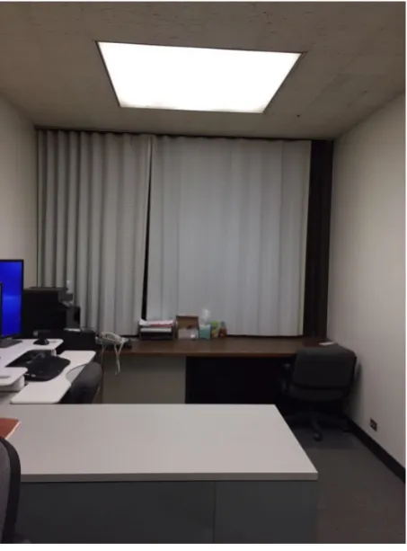
[image:2.595.319.546.79.386.2]

The present work was conducted to examine the thermal comfort performance of a private office during summer and winter at the University of Cincinnati (UC) (See Figure 1). Extensive CFD studies were performed based on the ventilation simulation software Autodesk® CFD. The entire CFD process consisted of the following steps. First, a geometric model was built. Next, the physical characteristics of the system were set, including materials, boundary conditions, and meshing. After that, a simulation was conducted based on an iterative calculation process. Finally, the results were retrieved and visualized. During this CFD procedure, the air flow satisfied the following three governing equations [13]:

Figure 1. A private office at UC

Conservation of mass

𝜕𝜕𝜕𝜕

𝜕𝜕𝑡𝑡+ 𝑢𝑢

𝜕𝜕𝜕𝜕

𝜕𝜕𝜕𝜕+ 𝑣𝑣

𝜕𝜕𝜕𝜕

𝜕𝜕𝜕𝜕+ 𝑤𝑤

𝜕𝜕𝜕𝜕

𝜕𝜕𝜕𝜕= 0 (1)

where 𝜌𝜌 is the density; and 𝑢𝑢, 𝑣𝑣, and 𝑤𝑤 are the 𝑥𝑥, 𝑦𝑦 and

𝑧𝑧 components of velocity, respectively. 2.1.1 Momentum Equations

𝑥𝑥- momentum equation:

𝜌𝜌𝜕𝜕𝜕𝜕_{𝜕𝜕𝑡𝑡}+ 𝜌𝜌𝑢𝑢𝜕𝜕𝜕𝜕_{𝜕𝜕𝜕𝜕}+ 𝜌𝜌𝑣𝑣𝜕𝜕𝜕𝜕_{𝜕𝜕𝜕𝜕}+ 𝜌𝜌𝑤𝑤𝜕𝜕𝜕𝜕_{𝜕𝜕𝜕𝜕}= 𝜌𝜌𝑔𝑔𝜕𝜕−𝜕𝜕𝜕𝜕_{𝜕𝜕𝜕𝜕}+_{𝜕𝜕𝜕𝜕}𝜕𝜕 �2𝜇𝜇𝜕𝜕𝜕𝜕_{𝜕𝜕𝜕𝜕}� +_{𝜕𝜕𝜕𝜕}𝜕𝜕 �𝜇𝜇 �𝜕𝜕𝜕𝜕_{𝜕𝜕𝜕𝜕}+𝜕𝜕𝜕𝜕_{𝜕𝜕𝜕𝜕}�� +_{𝜕𝜕𝜕𝜕}𝜕𝜕 �𝜇𝜇 �𝜕𝜕𝜕𝜕_{𝜕𝜕𝜕𝜕}+𝜕𝜕𝜕𝜕_{𝜕𝜕𝜕𝜕}�� + 𝑆𝑆𝜔𝜔+ 𝑆𝑆𝐷𝐷𝐷𝐷 (2) 𝑦𝑦- momentum equation:

𝜌𝜌𝜕𝜕𝜕𝜕_{𝜕𝜕𝑡𝑡}+ 𝜌𝜌𝑢𝑢𝜕𝜕𝜕𝜕_{𝜕𝜕𝜕𝜕}+ 𝜌𝜌𝑣𝑣𝜕𝜕𝜕𝜕_{𝜕𝜕𝜕𝜕}+ 𝜌𝜌𝑤𝑤𝜕𝜕𝜕𝜕_{𝜕𝜕𝜕𝜕}= 𝜌𝜌𝑔𝑔𝜕𝜕−𝜕𝜕𝜕𝜕_{𝜕𝜕𝜕𝜕}+_{𝜕𝜕𝜕𝜕}𝜕𝜕 �𝜇𝜇 �𝜕𝜕𝜕𝜕_{𝜕𝜕𝜕𝜕}+𝜕𝜕𝜕𝜕_{𝜕𝜕𝜕𝜕}�� +_{𝜕𝜕𝜕𝜕}𝜕𝜕 �2𝜇𝜇𝜕𝜕𝜕𝜕_{𝜕𝜕𝜕𝜕}� +_{𝜕𝜕𝜕𝜕}𝜕𝜕 �𝜇𝜇 �𝜕𝜕𝜕𝜕_{𝜕𝜕𝜕𝜕}+𝜕𝜕𝜕𝜕_{𝜕𝜕𝜕𝜕}�� + 𝑆𝑆𝜔𝜔+ 𝑆𝑆𝐷𝐷𝐷𝐷 (3) 𝑧𝑧- momentum equation:

𝜌𝜌𝜕𝜕𝜕𝜕_{𝜕𝜕𝑡𝑡} + 𝜌𝜌𝑢𝑢𝜕𝜕𝜕𝜕_{𝜕𝜕𝜕𝜕}+ 𝜌𝜌𝑣𝑣𝜕𝜕𝜕𝜕_{𝜕𝜕𝜕𝜕}+ 𝜌𝜌𝑤𝑤∂𝜕𝜕_{𝜕𝜕𝜕𝜕} = 𝜌𝜌𝑔𝑔𝜕𝜕−𝜕𝜕𝜕𝜕_{𝜕𝜕𝜕𝜕}+_{𝜕𝜕𝜕𝜕}𝜕𝜕 �𝜇𝜇 �𝜕𝜕𝜕𝜕_{𝜕𝜕𝜕𝜕}+𝜕𝜕𝜕𝜕_{𝜕𝜕𝜕𝜕}�� +_{𝜕𝜕𝜕𝜕}𝜕𝜕 �𝜇𝜇 �𝜕𝜕𝜕𝜕_{𝜕𝜕𝜕𝜕}+𝜕𝜕𝜕𝜕_{𝜕𝜕𝜕𝜕}�� +_{𝜕𝜕𝜕𝜕}𝜕𝜕 �2𝜇𝜇𝜕𝜕𝜕𝜕_{𝜕𝜕𝜕𝜕}� + 𝑆𝑆𝜔𝜔+ 𝑆𝑆𝐷𝐷𝐷𝐷 (4)

The two source terms, 𝑆𝑆𝐷𝐷𝐷𝐷 and 𝑆𝑆𝜔𝜔, in the momentum equations represent the rotating coordinates and distributed

resistances respectively. The distributed resistance term, 𝑆𝑆𝐷𝐷𝐷𝐷, can generally be written as:

𝑆𝑆𝐷𝐷𝐷𝐷= − �𝐾𝐾𝑖𝑖+_𝐷𝐷𝑓𝑓_𝐻𝐻�𝜕𝜕𝑉𝑉𝑖𝑖 2

2 − 𝐶𝐶𝜇𝜇𝑉𝑉𝑖𝑖 (5)

where 𝑖𝑖 refers to the global coordinate direction (𝑢𝑢, 𝑣𝑣, and 𝑤𝑤 in the momentum equation). The 𝐾𝐾-factor term can operate only in a single momentum equation at a time because each direction has its own unique 𝐾𝐾-factor. The other two resistance types operate equally in each momentum equation.

The other source term represents rotating flow. This term can generally be written as:

(3)

where 𝑖𝑖 refers to the global coordinate direction, 𝜔𝜔 is the rotational speed and 𝑟𝑟 is the distance from the axis of rotation. 2.1.2. Energy E_{quation (Temperature Form)}

For incompressible air flow, the energy equation can be written in terms of static temperature:

𝜌𝜌𝐶𝐶𝜕𝜕𝜕𝜕𝜕𝜕_{𝜕𝜕𝑡𝑡}+ 𝜌𝜌𝐶𝐶𝜕𝜕𝑢𝑢𝜕𝜕𝜕𝜕_{𝜕𝜕𝜕𝜕}+ 𝜌𝜌𝐶𝐶𝜕𝜕𝑣𝑣𝜕𝜕𝜕𝜕_{𝜕𝜕𝜕𝜕}+ 𝜌𝜌𝐶𝐶𝜕𝜕𝑤𝑤𝜕𝜕𝜕𝜕_{𝜕𝜕𝜕𝜕}=_{𝜕𝜕𝜕𝜕}𝜕𝜕 �𝑘𝑘𝜕𝜕𝜕𝜕_{𝜕𝜕𝜕𝜕}� +_{𝜕𝜕𝜕𝜕}𝜕𝜕 �𝑘𝑘𝜕𝜕𝜕𝜕_{𝜕𝜕𝜕𝜕}� +_{𝜕𝜕𝜕𝜕}𝜕𝜕 �𝑘𝑘𝜕𝜕𝜕𝜕_{𝜕𝜕𝜕𝜕}� + 𝑞𝑞𝑉𝑉 (7)

where 𝐶𝐶𝜕𝜕 refers to the constant pressure the specific heat, 𝑘𝑘 is the thermal conductivity, 𝑇𝑇 is the temperature, and 𝑞𝑞𝑉𝑉 is the

volumetric heat source.

2.2. CFD Modelling 2.2.1. Geometric Model

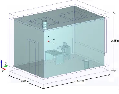
A geometric model of the private office simulated for this study can be found in Fig. 2. The dimensions of the private office were 4.57m × 3.05m × 3.05m (clear length × clear width × clear height). The door’s dimensions were 2.18m × 0.91m (height × width). The window’s dimensions were 2.13m × 2.99m (height × width). The thickness of the wall was 0.20m. The thickness of the ceiling and floor were both 0.30m. The radius of the duct was 0.15m and the terminal dimensions was 0.30m × 0.30m. There were two lamps located on the ceiling; their box dimensions were 1.22m × 1.22m. The one supply vent inlet was in the middle of the wall, under the bottom of the window; the one return outlet was located close to and above the door

.

2.2.2. Material Setting

[image:3.595.209.404.405.559.2]

Base on the real data for the office and the requirements in ASHRAE 90.1-2013, we assigned different materials to every part of the private office model (see Table 1). We defined the materials for “External Wall”, “Floor tiles”, “Wood (door)”, and “Window Glass” in the Autodesk® CFD software because these materials were not included in its materials database. Among the building envelope associated assemblies, windows can contribute significantly to the energy consumption and indoor thermal conditions [14]. In order to explore the potential differences, we adopted regular air-filled double pane glazing which is normally used in offices [15].

Figure 2. Geometric model of the private office

Table 1. Material Properties of the Private Office Depicted in the CFD Model

Part Material Emissivity Conductivity Density W/m-_K _{kg/ m}3

External wall External wall 0.8 0.07 2306 Interior wall Gypsum board 0.8 0.17 800

Ceiling Gypsum board 0.8 0.17 800

Floor Floor tiles 0.85 1.5 800

Door Wood (door) 0.8 0.58 510

Window Window glass 0.92 0.49 2700

Furniture Wood (soft) 0.8 0.12 510

Laptop Aluminum alloy (6061) 0.2 180 2700

Lamp Acrylic 0.5 0.19 1190

Human Human 0.98 50 998

[image:3.595.61.550.588.744.2]

(4)

2.2.3. Boundary Conditions

Two supply boundary conditions were set for the summer and the winter scenarios. In Autodesk® CFD, the supply-side conditions were configured according to a volume flow rate of 0.047m3_{/s; the supply temperature was} 20℃ in summer and 38℃ in winter. The return boundary condition was defined as a pressure equal to 0, since we were using a pressure gauge condition to represent the exhaust air in the return ducts. In both scenarios, there was no shade.

For the summer scenario, the external conditions were modelled with a film coefficient of 8.29W/m2_{K for the} external wall, 3.35W/ m2_{K for the window; this simulated air} movement from natural convection only, the outside temperature of the office was 35℃, so the reference temperature was 35℃. Regarding the winter scenario, the film coefficients were kept the same as the values in the summer scenario, and the reference temperature was -15℃. In addition, there were three heat sources in the studied office, including the following:1) a metabolic heat power 130W of one faculty, 2) radiated heat of 130W from the laptop, and 3) a dissipated heat power of 100W from each lamp.

2.3. Thermostat Settings

We considered a mixed convection and used a 𝑘𝑘 − 𝜀𝜀

turbulence model in this study. We employed a transient simulation to observe the office cooling down or heating up to a comfortable temperature when the user arrived. We set the air handler fan to be turned off when the thermostat sensed that the temperature was lower than 24℃in the summer or higher than 21℃ in the winter. In addition, buoyancy effects and solar radiation were not considered in this simulation study.

Thermostats are often located on interior walls near work zones, and mostly operated by static set-point controls or

schedule-driven building automation systems [16]. In this research, the thermostat was placed on the wall close to the user’s position, at a height of 1.6m from the floor. Then, we set up a monitoring point using the thermostat’s geometric position to track and monitor the temperature (see the red point in Fig. 2). The data from the monitoring point were available in the output bar and could be visualized while the solution was in progress.

3. Temperature Variations

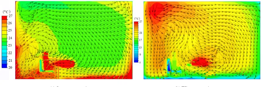
The simulation results of the temperature distributions across a vertical plane that passed through the location of the occupant in the summer and winter scenarios are shown in Figs. 3 and 4. The temperature distributions across a horizontal plane that passed through the location of the occupant in the summer and winter scenarios were also generated by the simulation and are extracted in Figure 4. In order to avoid local discomfort, ANSI/ASHRAE Standard 55-2013 recommends that the air temperature difference between the 0.1 and 1.1m height levels should be less than 3℃, and the air temperature difference between the 0.1 and 1.7m height levels should be less than 4℃. Therefore, we also extracted the air temperatures at three height levels (0.1m, 1.1m, and 1.7m) to calculate the vertical temperature differences in the user-occupied zone; these data are generalized in Table 2.

From Figures 3 and 4, we can see that the highest temperature occurred at the occupant’s position and at floor level, close to the door. The overall air temperature distribution was not uniform across both the vertical or horizontal planes.

[image:4.595.82.530.506.654.2]

(a) Summer scenario (b) Winter scenario

(5)

[image:5.595.81.532.77.216.2]

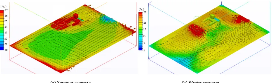
(a) Summer scenario (b) Winter scenario

Figure 4. Horizontal distribution of temperatures

[image:5.595.55.297.533.607.2]

In summer (Fig. 3a and 4a), the floor-level airflow moved to emanate uniformly from the supply. The air velocity was almost constant in the room at this level, and was generally below 0.01m/s. The velocity was higher and uneven in the vicinity of the air supply terminal. The air supply register could not fully merge the hot air around the window with the cool air coming from the air supply register. In Table 2, the vertical temperature difference at the occupant position between 0.1m and 1.1m was 1.6℃, and the vertical temperature difference at the occupant position between 0.1m and 1.7m was 2.3℃. These values complied with the ASHRAE 55 recommendation. In the winter scenario (Fig. 3b and 4b), the temperature differences increased. The airflow patterns showed that the cool air around the window was fully and quickly merged with the hot air from the supply air register. There was almost no direct airflow from the cold side of the window. It should be noted that the vertical temperature between 0.1m and 1.1m was 4.4℃ (see Table 2), and the vertical temperature difference at the occupant position between 0.1m and 1.7m was 4.7℃. These vertical temperature gradients were above the ASHRAE 55 recommended limits.

Table 2. Temperature Differences in Summer and Winter Scenarios Summer Winter Temperature at the thermostat 24℃ 21℃

Vertical temperature difference (0.1-1.7m) 2.3 4.7 Vertical temperature difference (0.1-1.1m) 1.6 4.4 Horizontal temperature difference (min vs. max) 8 10

In addition, we determined the temperature distribution across the horizontal plane. This showed that the horizontal temperature difference (maximum vs. minimum) was 8℃

and 10℃ for summer and winter, respectively. Such large horizontal temperature variations might also negatively affect users’ indoor comfort.

These results for the thermal distribution simulation revealed a clear spatial variation across both the vertical and horizontal planes, because the thermostat was not located in the user-occupied zone. Therefore, although the temperature conditions at the thermostat were within the comfortable range, the occupant might still have felt different thermal

conditions when in different locations around the office. The spatial variations in temperature (2.3/1.6/8℃ in summer and 4.7/4.4/10℃ in winter) would cause the occupant to feel thermal discomfort.

4. PMV-PPD

Using Autodesk CFD, the PMV index could also be also calculated and visualized in a 3D view (see Figure 5). The PMV index provides more meaningful information regarding thermal comfort than does air temperature. PMV is divided into a seven-point thermal sensation scale, according to the thermal perception of the human body (+3 hot, +2 warm, +1 slightly warm, 0 neutral, -1 slightly cool, -2 cool, -3 cold) [8]. We extracted the PMV indices for two points at a head-level of 1.1m and foot-level of 0.1m from the simulation scenarios, and then obtained the average PMV values. Also, to predict the percentile of individuals who would be thermally dissatisfied in a given environment, the Predicted Percentage of Dissatisfied (PPD) index was calculated using Eq. (8), and the data were analyzed [15]. Table 3 summarizes the two key thermal comfort indicators obtained in this simulation study.

PPD = 100 − 95 ∙ 𝑒𝑒−�0.03353∙𝑃𝑃𝑃𝑃𝑉𝑉4+0.2179∙𝑃𝑃𝑃𝑃𝑉𝑉2�₍₈₎

In this research, air conditioning was stopped once the air temperature at the thermostat position reached 24℃ and 21℃

(6)

(-0.5) occurred near the head and right side of the occupant’s body; the minimum PMV (-3) was found near the left foot of the body scale [7].

The recommended acceptable PPD range from ANSI/ASHRAE Standard 55-2013 is less than 10% of persons dissatisfied with the interior space [17]. Even though the PMV and PPD values at the thermostat position were ideally preferable, the conditions in the user zone were still outside of the recommended limits. The PPD values found in this study were higher – about 6.8% and 2.6% in summer and winter, respectively – than this limit. In other words, conditions controlled by a wall-mounted thermostat might result in user discomfort.

(a) Summer scenario

(b) Winter scenario

[image:6.595.81.274.246.638.2]

Figure 5. Predicted mean vote for the office

Table 3. PMV-PPD Indicators

Summer Winter PMV at thermostat 0 0

Average PMV 0.75 -0.6 Average PPD (%) 16.8 12.6

5. Conclusions

The spatial variations in temperature and thermal comfort PMV-PPD index in a typical office were simulated and analyzed using Autodesk® CFD simulation techniques. The visualized thermal conditions were presented in this paper.

In this study, the successful application of Autodesk® CFD suggests that this method can provide useful, efficient, and easily visualized information useful in analyzing indoor thermal comfort. The main conclusions that can be drawn from this study are as follows:

The numerical simulation results verified our hypothesis regarding the effects on thermal variation and potential thermal discomfort stemming from the use of a wall-mounted thermostat in a typical private office. In particular, thermostats are normally installed on walls rather than at occupant positions, so the temperature values sensed do not reflect the actual air temperature of the occupied space in the office. Accordingly, the temperature of the thermostat is not representative of the room temperature; the result is a temperature difference between the height levels within the occupied space that may exceed the recommended thermal comfort limits. In this research, in summer, when the thermostat arrived at a comfortable temperature of 24℃, the vertical temperature difference between what was measured at 0.1m and 1.1m was 2.3℃; moreover, the vertical temperature difference at the occupant position between 0.1m and 1.7m was 1.6℃. In the winter, when the thermostat arrived at a comfortable temperature of 21℃, the vertical temperature between 0.1m and 1.1m was 4.4℃; the vertical temperature difference at the occupant position between 0.1m and 1.7m was 4.7℃. These vertical temperature gradients exceed the ASHRAE 55 recommended limits [18]. At the same time, the horizontal temperature differences (maximum vs. minimum) were 8℃ and 10℃ for summer and winter, respectively. Consequently, people in the occupied spaces would not have felt as comfortable as they would have if the actual temperature was that which was reflected by the thermostat’s received temperature value.

(7)

REFERENCES

[1] ASHRAE 90.1. Energy standard for buildings except low-rise residential buildings. American Society of Heating, Refrigerating and Air-Conditioning Engineers (ASHRAE), 2013.

[2] A. Wagner, E. Gossauer, C. Moosmann et al. Thermal comfort and workplace occupant satisfaction-results of field studies in German low energy office buildings, Energy and Buildings, Vol.39, No.7, 758-769, 2007.

[3] A. Alajmi, F. Baddar, and R. Bourisli. Thermal Comfort Assessment of an Office Building Served by under-Floor Air Distribution (UFAD) System - A Case Study. Building and Environment, Vol. 85, 153–159, 2015.

[4] A. Melikov and J. Nielsen. Local Thermal Discomfort due to Draft and Vertical Temperature Difference in Rooms with Displacement Ventilation. ASHRAE Transactionsz: Research, Vol.95, 1989.

[5] B. Olesen, M. Scholer, and P. Fanger. Discomfort Caused by Vertical Air Temperature Differences. Indoor Climate, Vol. 36, 561-579, 1979.

[6] D. Wvon and M. Sandberg. Discomfort due to Vertical Thermal Gradients. Indoor Air, Vol. 6, No.1, 48-54, 1996.

[7] B. Olesen and G. Brager. A better way to predict comfort. ASHARE Journal, August, 20-26, 2004.

[8] J. Moon and S. Han. Thermostat strategies impact on energy consumption in residential buildings. Energy and Buildings, Vol.43, No. 2-3, 338-346, 2011.

[9] S. Al-Sanea and M. Zedan. Optimized monthly-fixed thermostat-setting scheme for maximum energy-savings and thermal comfort in air-conditioned spaces. Applied Energy, Vol.85, No.5, 326-346, 2008.

[10]J. Moon, J. Chang and S. Kim. Determining Adaptability Performance of Artificial Neural Network-Based Thermal

Control Logics for Envelope Conditions in Residential Buildings. Energies, Vol. 6, No. 7, 3548–3570, 2013.

[11]J. Sengupta, K. Chapman and A. Keshavarz. Window Performance for Human Thermal Comfort. ASHRAE Transactions: Research, Vol. 111, No.1, 254-275, 2005. [12]Q. Duan, J. Wang and H. Zhao. Airflow pattern and thermal

comfort in winter by different combinations of air distribution strategies and window types in an office unit. The Passive Low Energy Architecture Conference, Edinburgh, UK, 2017. [13]Autodesk CFD Help. General Fluid Flow and Heat Transfer

Equations. Online available from

https://knowledge.autodesk.com/support/cfd/learn-explore/ca as/CloudHelp/cloudhelp/2014/ENU/SimCFD/files/GUID-83 A92AE5-0E9E-4E2D-B61F-64B3696E5F66-htm.html [14]J. Wang, L. Caldas, D. Chakraborty, and L. Huo. Selection of

energy efficient windows for hot climates using genetic algorithms optimization. In Proceedings of PLEA 2016, International Conference on Passive and Low Energy Architecture 2016: Cities, Buildings, People: Towards Regenerative Environments, Los Angeles 2016 Jul 11. [15]W.J. Hee, M.A. Alghoul, B. Bakhtyar, O. Elayeb, M.A.

Shameri, M.S. Alrubaih, and K. Sopian. The role of window glazing on daylighting and energy saving in buildings. Renewable and Sustainable Energy Reviews, 42, pp.323-343. [16]S. Carmichael, C. Booten and J. Robertson et al. Annual

energy savings and thermal comfort of autonomously heated and cooled office chairs. National Renewable Energy Laboratory, Technical Report. July, 2016.

[17]ISO-7730. Ergonomics of the thermal environment-analytical determination and interpretation of thermal comfort using calculation of the PMV and PPD indices and local thermal comfort criterial. International Organization for Standardization, Geneva, Switzerland. 2005.