Studies of labor market data

(1)

THELONDON SCHOOL OFECONOMICS AND POLITICALSCIENCE

Studies of Labor Market Data

F

ELIX

N

IKOLAUS

K

OENIG

A

THESIS SUBMITTED TO THE

D

EPARTMENT OF

E

CONOMICS OF THE

L

ONDON

S

CHOOL OF

E

CONOMICS FOR THE DEGREE OF

D

OCTOR OF

(2)

Declaration

I certify that the thesis I have presented for examination for the MPhil/PhD degree of the London School of Economics and Political Science is solely my own work other than where I have clearly indicated that it is the work of others (in which case the extent of any work carried out jointly by me and any other person is clearly identified in it).

The copyright of this thesis rests with the author. Quotation from it is permitted, provided that full acknowledgment is made. This thesis may not be reproduced without the prior written consent of the author.

I warrant that this authorisation does not, to the best of my belief, infringe the rights of any third party.

I declare that this thesis consists of approximately 38,000 words.

Statement of inclusion of previous work

I confirm that work on Chapter 3 began prior to my enrollment in the PhD. The research paper has not been submitted for any prior degree.

Statement of conjoint work

I confirm that Chapter 2 was jointly co-authored with George Fenton and I contributed 50% of this work and Chapter 3 was jointly co-authored with Professor Alan Manning and Professor Barbara Petrongolo and I contributed 33%.

Statement of use of third party for editorial help

I confirm that parts of Chapter 1 of this thesis was copy edited for conventions of language, spelling and grammar by Kaley Joyce and Michael Beaney and Sarah Taylor of the LSE language centre.

(3)

Abstract

The thesis uses micro data and quasi experimental research designs to test three theories about labor markets.

The first chapter tests a leading explanation for top income growth, the superstar effect. The superstar effect attributes rising top incomes to expanding market reach of workers. I identify a case of exogenous market reach expansion in the entertainment sector and study the labor market effects. Incomes become markedly more concentrated on the top when entertainers can reach a bigger audience. Wages of stars grow 17% in response to a fourfold increase in market reach. A distinctive pattern of wage changes distinguishes the superstar model from alternative explanations. Growth of top pay occurs simultaneously with widening income differences at the top, a decline in middle-income jobs, an increase in low-paid jobs and a fall in total entertainer employment.

The second chapter tests how labor supply responds to improving entertainment technology. To identify the effect the chapter tracks the roll-out of TV signal. Social security records show that labor supply drops significantly with the introduction of TV. The effects are most pronounced for older workers, in line with descriptive evidence on changing retirement habits. The chapter shows that monetary spending substantially understates the value attached to TV.

The third chapter studies the canonical search and matching model and shows that accounting for realistic job search helps the model to account for labor market fluctuations and addresses the “Shimer puzzle.” The chapter provides evidence that reservation wages significantly respond to backward-looking reference points. Introducing such reference-dependent job search to the model reconciles predictions on the cyclicality of both wages and reservation wages with the data. Other proposed solutions to the unemployment volatility and wage flexibility puzzle that hinge on alterations to the wage setting mechanism only work for parameter values outside the range typically estimated.

(4)

Acknowledgments

This thesis relied on the support of a great number of people.

Foremost, I thank my supervisor Steve Pischke, who has been a fantastic role model and supported and challenged me in countless ways throughout my PhD. I am particularly appreciative for the countless hours we spent with the all the projects that got discarded on the way.

Another key ingredient to this thesis was the fantastic research environment and outstanding academics at LSE and MIT. I am particularly grateful to David Autor and Alan Manning. David has been an amazing source of inspiration for the last two years. Thanks for your enthusiasm, attention to detail and your round the clock availability. And to Alan for the light hearted approach to research and the fun anecdotes that spiced up many research projects.

My co-authors and peers have been a crucial source of encouragement. Seeing projects through has been a breeze together with George Fenton, Barbara Petrongolo and John van Reenen. Just as valuable was the research community at CEP. Particular thanks goes to Jan Baker, Catherine Thomas, Vincenzo Scrutinio and Anna Valero who were incredibly helpful in drafting this research.

Without doubt, my PhD peers had the biggest impact on this thesis. The foundation for this thesis was laid during many problem set sessions and philosophical coffee breaks with Thomas Drechsel, Friedrich Geiecke, Niklas Moneke and Claudio Schilter. The joint supervisory meetings with Andres Barrios, Giulia Bovini, Giulia Giupponi and Stephan Maurer were invaluable and thanks for those shared memories of break-throughs, set-backs and frustrations. At least as important were the wind-down moments in the gym, pool and in the saddle with Wolfgang Ridinger, Thomas St¨ork, Arthur Seibold and Torsten Figueiredo Walter.

I am also grateful to the people who welcomed me during my research visits at Goethe University and MIT. To Horst Entorf for offering unconditional support during a difficult period, to Magda Davoli and Sunny Dutt for fantastic company at Campus West End. Thanks to Josh Angrist for hosting me in Cambridge and for being Master Joshway on the mountain bike trails. Thanks to my MIT office mates and the labor group, among others Jacob Moscona, Marco Tabellini, Camille Terrier, Joonas Thukuri, Matthias Wilhelm and Samy Young, the MIT cycling club and my flat mates for introducing me to the BSO, facial conducting and life in Cambridge.

Most of all I am indebted to my family. Foremost to Victoria who has kept me sane, cheered me up and has been the best company I could have wished for. To Anne, Lothar and Franca without whom I would not have made it to and through university. To the Russos and Richardsons, the past years would not have been the same without our amazing travels, bike rides and messages from every corner of the world.

Finally, I am grateful for financial support from the Economic and Social Research Council.

(5)

The Labor Supply Response to Entertainment Technology

114

9 Introduction 114 10 Measuring TV Access 117 10.1 The Irregular Terrain Model . . . 117

10.2 Television FactbookData . . . 117

10.3 Visualizing the ITM . . . 118

11 Labor Supply Data 119 11.1 Individual Social Security Records . . . 119

11.2 County-Level Census Data . . . 119

12 Design and Analysis 120 12.1 Results: Individual Social Security Records . . . 121

12.2 Results: County-level Census Data . . . 122

12.3 Placebo Tests . . . 124

12.4 Terrain Variation . . . 124

12.5 Heterogeneous Effects: The Role of Retirement . . . 125

13 Welfare Estimates 126 14 Conclusion 128 15 Appendix II 130 15.A Tables . . . 130

15.B Figures . . . 134

15.C The DMA Approximation . . . 140

15.D Additional Tables and Figures . . . 143

III

Reservation Wages and the Wage Flexibility Puzzle

149

16 Introduction 149 17 The model 152 17.1 Employers . . . 152

17.2 Workers . . . 154

(7)

17.3 Wage determination . . . 154

17.4 The reservation wage . . . 155

18 The Predicted Cyclicality of Wages 157 18.1 A comparison of steady states . . . 157

18.2 The General Case . . . 160

18.3 Benchmark parameters . . . 164

18.4 Case I: Continuous Wage Negotiation . . . 166

18.5 Case II: No backward-looking component in wage determination . . . . 166

18.6 Case III: Infrequent Wage Negotiation and Backward-Looking Wages . 167 18.7 Reference-dependence in Reservation Wages . . . 168

19 Empirical wage and reservation wage curves. 170 19.1 Estimates of the wage curve . . . 170

19.2 Estimates of the reservation wage curve . . . 172

19.3 The quality of reservation wage data . . . 174

20 Reference dependence in reservation wages 175 20.1 Quantitative predictions of reference dependence . . . 178

21 Conclusions 179 22 Appendix III 181 22.A Tables . . . 181

22.B Figures . . . 188

22.C Derivation of model results . . . 193

22.D Additional Tables and Figures . . . 208

22.E Alternative models for the reservation wage . . . 215

(8)

List of Tables

Appendix I 50

1 Effect of TV on Entertainer Top Earners . . . 50

2 Effect of TV on Market Reach of Local Stars . . . 51

3 Effect of TV on Log Spending at Local County Fairs . . . 52

4 Effect of TV on Entertainer Employment. . . 53

5 Effect of TV on Top Income Shares in Entertainment . . . 54

6 Effect of TV on Mobility Between Labor Markets . . . 55

7 Elasticity of Entertainer Top Pay to Market Reach . . . 56

8 Effect Heterogeneity by Market Structure . . . 57

9 Effect of TV on Top Earner - Placebo Occupations . . . 107

10 Effect of TV on Top Earner - Alternative Top Income Measures . . . . 108

11 Alternative Top Income Measures . . . 109

12 Effect of TV on Top Earner - Micro Data. . . 110

13 Effect of TV on Top Earner - State Level . . . 111

14 Earning Effect - triple diff. . . 112

15 Quantile Effect of TV . . . 112

16 Small Sample Performance of Pareto Shape Parameter Estimators . . . 113

17 Policy Effects in a Superstar Setting . . . 113

Appendix II 130 18 Effect of TV on Labor Supply - Individual Level . . . 130

19 Effect of TV on Labor Supply - County Level . . . 131

20 Placebo Test with Blocked TV Channels . . . 131

21 Heterogeneous Effects . . . 132

22 Willingness to Pay for TV . . . 133

23 Proximal Market Areas . . . 144

Appendix III 181 24 Benchmark Parameters for the UK and West Germany . . . 182

25 Estimates of a Wage Equation for the UK, 1991-2009.. . . 183

26 Estimates of a Wage Equation for the West Germany, 1984-2010 . . . . 184

27 Estimates of a Reservation Wage Equation for the UK, 1991-2009. . . . 185

28 Estimates of a Reservation Wage Equation for West Germany, 1987-2010.185 29 Reservation Wages, Post-Unemployment Wages and Job Finding Prob-abilities in the UK, 1991-2009 . . . 186

30 Reservation Wages, Post-Unemployment Wages and Job Finding Prob-abilities in West Germany, 1987-2010 . . . 186

31 Reservation wages and rents in previous jobs: UK, 1991-2009. . . 187

32 Descriptive statistics . . . 209

(9)

33 Detailed results on wage and reservation wage equations for the UK and West Germany . . . 210

34 Estimates of a Wage Equation for the UK, 1991-2009. Further estimates with regional controls. . . 211

35 Estimates of a Wage Equation for West Germany, 1984-2010. Further estimates with regional controls . . . 212

36 Estimates of a Reservation Wage Equation for the UK, 1991-2009. Further estimates with regional controls. . . 213

37 Estimates of a Reservation Wage Equation for West Germany. Further estimates with regional controls . . . 214

38 The Cyclicality in the Fraction of New Hires from Previously Jobs . . . 218

(10)

List of Figures

Appendix I 50

1 Effect of Technical Change on Wage Distribution – Superstar Model . . 58

(a) Wage Distribution . . . 58

(b) Employment Growth at Different Wage Levels . . . 58

2 Effect of Technical Change on Wage Distribution – Skill Biased Demand Model . . . 59

3 Intensity of TV Filming in 1949 . . . 60

4 TV Signal of Licensed and Frozen Stations in 1949 . . . 61

5 Entertainer Wage Distribution 1940 and 1970 . . . 62

6 Entertainment Employment per Capita . . . 63

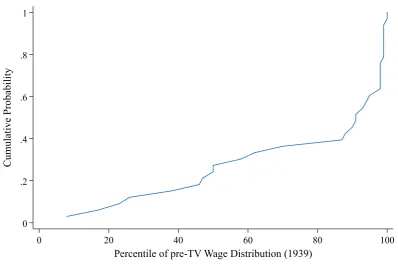
7 Position of Future TV Stars in the 1939 US Wage Distribution . . . 64

8 Number of TV Licenses Granted . . . 65

9 Dynamic Treatment Effect of TV on . . . 66

(a) Blocked TV Stations . . . 66

(b) Active TV stations . . . 66

10 Effect of TV on Entertainer Employment Growth at Different Wage Levels 67 11 Superstar Wage Distribution . . . 99

12 Effect of Technical Change on Wage Distribution - Skill Biased Demand Model . . . 100

13 Superstar Effect on Top Earner . . . 101

14 Theatre Seating Capacity . . . 102

15 P95-P50 Gap . . . 103

16 Top Income Percentile Values . . . 103

17 Dynamic Treatment Effect of TV stations - Placebo Occupations . . . . 104

18 Quantile Effects of Television . . . 105

Appendix II 130 19 Average Hours of TV per Day in the US . . . 134

20 1948 ITM Signal Strength . . . 135

24 Effect of TV on Leisure: Percent Not Working . . . 137

25 Effect of TV on Leisure: Quarters Worked . . . 137

26 Leisure Response to more TV Channels . . . 138

27 Number of TV Station Construction Permits Issued . . . 138

28 TV Signal of Licensed and Frozen Stations . . . 139

29 Treatment Effect by Age Groups . . . 139

30 Coverage Maps and Designated Market Areas . . . 145

(11)

31 TV Purchases Patterns . . . 146

32 Broadcast Tower Improvements . . . 147

33 ITM Signal Strength, Kansas City and Minneapolis-St. Paul . . . 148

Appendix III 181

34 The role of backward looking behaviour in wage setting (1−α) and

frequency of wage renegotiations (φ) in wage and reservation wage

cyclicality. UK parameter values. . . 188

35 The role of backward looking behaviour in wage setting (1−α ) and

frequency of wage renegotiations (φ ) in wage and reservation wage

cyclicality. West Germany parameter values. . . 189

36 The role of reference dependence in reservation wages (1−αρ ) on

wage and reservation wage cyclicality. UK parameter values. . . 190

37 The role of reference dependence in reservation wages (1−αρ ) on

wage and reservation wage cyclicality.West Germany parameter values. 191

38 Parameter Values that Explain Observed Cyclicality . . . 192

(12)

Introduction

This thesis consists of three chapters that study the functioning of labor markets. Over the past 60 years labor markets have changed dramatically. Two of the most striking trends are the decline in labor market participation and the sharp increase in income inequality. Economists have used models to shed light on the mechanisms that may drive these trends. In this thesis I test three prominent models empirically.

The three chapters use the same methodological approach and apply micro data and modern empirical methods to test hypothesis derived from economic models. The empirical tests use quasi-experimental tools to establish causal effects. The work thus combines empirical work with economic theory, which allows me to highlight the strength as well as areas of misspecification in prominent models of the labor market. The first chapter focus on the wage distribution and tests a leading theory of top income growth - “the superstar theory”; while the second and third chapter focus on explanation for changes to employment. The latter two chapters respectively study the search and matching model and the labor-leisure trade-off.

The first chapter studies top income growth and focuses on a leading explanation for such growth, the so called superstar effect. I present a tractable version of the model to illustrate the implication of the superstar effect. I then show how periods of expanding market reach of workers can be used to distinguish superstar effects from conventional models of labor markets. I use a historic period of location specific expansions in market reach in the entertainment sector to test the key predictions of the superstar model. Newly collected data on the licensing process of TV filming allows me to identify locations where the launch of television filming is delayed for exogenous reasons. The locally staggered variation in market reach gives rise to a differences-in-differences setting which allows me to test the superstar model. My results show that expanding market reach moves local wage distributions closer to winner takes all markets. Wages at the 99th percentile grow 17% while mid-paid jobs disappear and overall employment falls. Specific predictions of the superstar model distinguish the superstar model from alternative channels and confirm that superstar effects are driving the results.

The second chapter tests how labor supply responds to improving entertainment technology. Entertainment has improved rapidly over the past decades. This paper shows that better home entertainment options have led to a substantial decline in labor supply, particularly among the elderly. To identify the effect, we track TV signal during the introduction in the US and exploit variation from a regulated roll-out and terrain interference. Social security records allow us to measure how individual level labor supply responds. Our results confirms descriptive evidence that better leisure activities contributed to changes in retirement habits over the twentieth century. Finally, we use our estimates to quantify the forgone income from watching TV. Our results show that monetary expenditure on TV represents only a small fraction of total expenditure on this technology. Spending based measures like GDP therefore underestimate the value

(13)

created by free-to-use technologies like TV.

The third chapter studies the currently dominant model of wage cyclicality, the search and matching model. The quantitative predictions of the canonical search model are at odds with the observed fluctuations in wages and employment in the labor market. We emphasize the role of reservation wages in wage cyclicality and argue that reference-dependence in reservation wages can reconcile model predictions and empirical evidence on the cyclicality of both wages and reservation wages. We provide evidence that reservation wages significantly respond to backward-looking reference points, as proxied by rents earned in previous jobs. We also argue that other proposed solutions to the unemployment volatility and wage flexibility puzzle that hinge on alterations to the wage setting mechanism only work for parameter values outside the range typically estimated.

(14)

Part I

Superstar Earners and Market Size:

Evidence from the Roll-Out of TV

1

Introduction

Rapid top income growth has been a striking feature of many labor markets in recent decades.1 One of the leading economic explanations for this type of change in the wage distribution is the superstar effect.2 According to this theory top income growth arises when workers can apply their talent on a bigger scale. As it gets easier to reach many consumers simultaneously, a greater share of consumers will flock to the most talented workers in the profession – the “superstars”. Such a shift in demand creates rising incomes at the top and simultaneously reduces incomes for less talented workers. The superstar effect can therefore explain why top incomes are growing much faster than average incomes and rationalize rapid top income concentration. This theory has a long tradition in economics and has been used widely to explain labor market trends, it has however rarely been tested.3

This paper uses a historic natural experiment to directly test the predictions of the superstar model. Workers are increasingly able to reach larger markets with the help of modern technologies. I use a historic setting to identify the effect of such changes on labor market returns and use it to test the superstar model. The entertainment sector provides a unique setting for such a test. The launch of TV in the mid 20th century had vastly increased the audience available to entertainers. Before the introduction of TV, a live performance could be watched by a few hundred individuals, while after the introduction of TV, the same performance could be watched by millions. Technological constraints limited TV filming to locations near broadcast antennas, as a result, TV was characterized by multiple local TV stations that independently broadcast content to the local population.4 For a local entertainer, the construction of a TV station was therefore 1_{For aggregate trends see}_{Alvaredo et al.}_{(2018); for occupation specific US data see}_{Kaplan and Rauh}

(2013);Bakija et al.(2012).

2_{Applications of the superstar model include}_{Gabaix et al.}_(2016);_Tervi¨o_(2008);_{Gabaix and Landier}

(2008);Garicano and Hubbard(2007);Cook and Frank(1995).

3_{Classic articles on the superstar model include}_Tinbergen_(1956);_Sattinger_(1975);_Rosen_(1981).

For a recent applications of this theory to the digital economy seeBas et al.(2018);Guellec and Paunov (2017);OECD(2016);Acemoglu et al.(2014).

4_{TV shows were effectively a non-tradable service. Recording was, in principle, possible in the form}

of “kinescopes.” However, the image quality of this technology was poor and such TV displays were unpopular. Shows produced elsewhere were a poor substitute for local productions. TV networks, which later harmonized programming across the US, initially had a limited influence over local programming.

(15)

a substantial shock to market reach, similar to the construction of a hypothetical giant theater that would hold an entire local population.

A growing number of local labor markets got access to TV filming during the staggered local deployment of TV stations. I study the effects of this roll-out in a difference in difference analysis across local entertainer labor markets and find that the launch of a TV station leads to sharp growth of top incomes, while simultaneously eroding demand for mediocre workers. The effects align closely with the superstar model but are at odds with conventional alternative models.

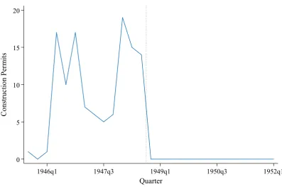
The roll-out of TV has exogenous elements that allow me to address three empirical challenges that made it difficult to test for superstar effects. A first challenge is that changes to market reach need to occur exogenously to local labor market shocks, which is rarely the case with ordinary endogenous technology adoption.5 In the case of TV on the other hand, technical change is introduced through a government licensing scheme. I exploit regulatory constraints to generate local variation in access to TV that is exogenous to local labor market conditions. One such feature is the sudden interruption of licensing in 1948 that became necessary due to signal interference between stations. I identify stations that were about to launch but narrowly missed out due to the license freeze. Such places that narrowly miss out on TV launches allow me to probe the identification assumptions and test for spurious effects in the government led roll-out process.

A second challenges is to isolate the effect of expanding market reach from other drivers of top income growth. The modern boom in market expanding technologies for example coincided with other trends that affect top incomes, such as deregulation and pay setting norms. The recent correlation of expanding market reach and top income growth may therefore reflect spurious effects. In the entertainment setting I can hold aggregate changes constant and exploit the fact that different parts of the US experience the effect at different times.

A third challenge for a test of superstar effects is that most innovations simultan-eously affect many aspects of the economy. Digital technologies, for instance, enable workers to serve bigger markets but also affect up and down stream markets, which makes it difficult to isolate the effect of worker market reach. TV, to the contrary, was used to broadcast entertainment shows and had no use in production of the rest of the economy. This allows me to isolate the effect of changing market reach from effects that occur in other industries.

A further advantage of the entertainment setting is that the entertainers’ audience size and it’s change through the TV roll-out can be quantified, overcoming one of the key measurement issues. I built a novel dataset from archival records that makes changes in production and consumption of entertainment visible. On the production 5_{Evidence for such endogenous technical change is presented in}_{Blundell et al.}_{(1999), the theory in}

Acemoglu(1998).

(16)

side, the data show where, when and why TV filming became feasible. Specifically, the data include information on the universe of broadcasting licenses of TV stations, their locations and audience sizes, as well as the historical capacity of over 3,000 performance venues. I combine this information with administrative records on the TV station licensing process, including information on how locations were prioritized. On the demand side, the data quantify the shift in labor demand. I digitize archival sources that report spending at roughly 4,000 local entertainment venues and contain information on prices and show revenues. With this data, I can trace demand shifts and associated changes in entertainers’ marginal revenue product. These records are linked to US Census micro-data that capture labor market outcomes in entertainment and beyond.

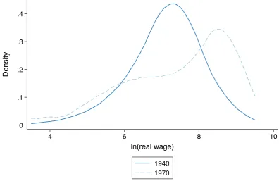
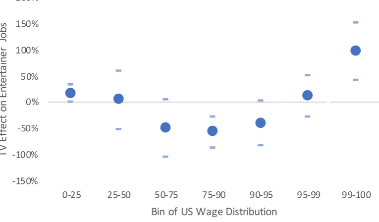
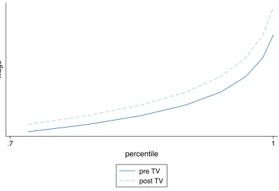
My findings confirm the headline prediction of the superstar model that growing market reach causes top income growth. A local TV station boosts pay at the 99th percentile by about 17% and expands the audience by roughly 300%. To put this wage growth into context, I look at the position of entertainers in the US wage distribution. Local star entertainers rise markedly in the US wage distribution when a TV station is launched in the labor market. The share of local entertainers in the top 1% of the US wage distribution almost doubles. Locations that narrowly miss out on the launch of a TV station see no growth in top entertainer pay. Similarly, I find no effect on other professions. The superstar effect is specific to the time periods, places and professions involved in local TV filming, reinforcing confidence that the effect is caused by TV.

Next, I show that the superstar effect differs from canonical models of technical change. To distinguish superstar effects, I derive additional predictions that are specific to the superstar model. In cross-sectional data, superstar effects and the effect of canonical labor demand shifts are indistinguishable. However, wage changes over time differentiates the superstar model from a wide range of alternative models. Specifically, in a superstar model labor markets move closer to a winner-takes-all market when it becomes easier for workers to reach a bigger market. These effects are captured by four testable predictions: (i) disproportionate wage growth at the top, (ii) decreasing wages for mediocre workers, (iii) falling employment and (iv) growing wage dispersion at the top. The empirical results confirm these patterns. Expanding market reach has a striking U-shaped effect across the wage distribution, characteristic of the superstar effect.6 The gains at the top occur together with a decline in mid-income jobs and a growing low-pay sector. Moreover, I confirm that low-pay differences among top earners increase and document substantial employment losses in entertainment. When TV signal becomes available in a local area, entertainment employment declines around 13%. These results show that demand is becoming concentrated on star workers, at the expense of mediocre 6_{The middle of the income distribution also hollows out in models of routinization where technology}

replaces mid-skilled workers (e.g.Goos et al.,2010). This differs from superstar models, where mid-skilled workers are replaced by star workers and technology acts as a vehicle for stars to project their talent.

(17)

workers.

Moreover, I can measure the shift in labor demand directly by studying spending data on different types of entertainment. This allows me to go beyond analyzing labor market outcomes and test the supposed underlying demand shift directly. The results show that local TV filming increases the audience and revenues for the biggest local shows while drastically reducing attendance at ordinary local live entertainment .

Next, I quantify the magnitude of superstar effects by estimating the elasticity of top pay to changes in market size. Data on audiences and prices allow me to measure market size in terms of the number of customers and revenues. I use this data in an instrumental variable (IV) strategy, where the launch of a TV station is the instrument for market size. This IV estimator shows that doubling audience size increases wages at the 99th percentile of entertainer pay distribution by 17%. The superstar effect can explain about 70% of differences in top incomes across local entertainer labor markets. An equivalent IV estimate that quantifies demand concentration in terms of revenues, finds a similar magnitude of superstar effects. As revenues become concentrated on top shows, 22 cents of each dollar go to top earners.

A potential concern with the empirical strategy is that the launch of a TV station is related to local trends that affect top pay in entertainment. I leverage the decline of local TV filming for a powerful parallel-trends test. The invention of videotape in 1956 made transporting and replicating shows attractive and led to modern production, in which shows are centrally produced and broadcast across the country. This resulted in the demise of local TV filming, and regional differences in the availability of production technologies therefore disappeared. As a consequence, local outcome differences ought to revert to their pre-treatment levels. This test goes beyond standard pre-trend checks, leveraging both pre- and post-treatment periods to verify common trends. The data confirms that the regulated TV roll-out is orthogonal to local trends.

Spillovers between local labor markets could bias estimates based on local labor markets relative to the effect of an aggregate shock. I assess such differences by studying spillovers between markets. A major spillover channel is shut-down in this setting since live entertainment shows are by nature consumed locally and there is no cross-labor market trade in output. The main potential link between local cross-labor markets is entertainer mobility. I quantify the mobility effects and find that they only play a minor role for the findings.

In a second extension, I explore how superstar effects interact with imperfect competition.7 The predictions of the superstar model change substantially in an imperfectly competitive labor market. Monopsony employers no longer pass on gains from technical progress to workers. The regulated entry of TV stations allows me to 7_{Imperfect competition features prominently in the market access literature. Integration of markets}

could give rise to entry effects that intensify competitive (Melitz and Ottaviano,2008). Monopsony power and rent-sharing have also been linked to pay inequality (e.g. Manning,2003;Benabou and Tirole,2016).

(18)

test this empirically and analyze how competition affects the magnitude of superstar effects. In line with the superstar model but contrary to popular belief, it is not the lack of competition that raises top incomes, but rather more intense competition for talent.8

The superstar model is a classic model in economics that was first presented six decades ago and became popular through a series of articles in the 70s and 80s that emphasized that the model could explain dramatic concentration of labor market returns at the top of the distribution (Tinbergen, 1956;Sattinger,1975;Rosen,1981). Despite this long tradition, there is no common modeling framework to study superstar effects. In an attempt to structure the literature, I develop a unifying framework that nests many of the existing superstar models (including Costinot and Vogel, 2010; Tervi¨o, 2008;

Gabaix and Landier,2008;Teulings,1995;Rosen,1981;Sattinger,1979,1975). I use a benchmark version of the model to show how improving production scalability affects the demand for talent and, ultimately, wages.9 Previous empirical applications use the superstar model to explain the distribution of CEO pay (Edmans and Gabaix, 2016;

Gabaix and Landier,2008;Tervi¨o,2008). Such studies calibrate key model parameters to the correlation of pay at the top and market size. My study instead focuses on distinguishing the superstar model from leading alternative models. In a link to the previous literature, I additionally provide a comparison of OLS and IV estimates for the key elasticities of the model.

A number of studies have shown that technical change has profound effects on labor markets. Canonical models of technical change include models of efficiency units (Stigler, 1961), skill biased technical change (Acemoglu and Autor, 2011; Katz and Murphy, 1992) and routine bias technical change (Acemoglu and Restrepo, 2018;

Autor and Dorn,2013;Goos et al.,2010). I show how the superstar model differs from such models and derive testable predictions that allow me to distinguish the models in the data. Empirical evidence for the canonical models use variation in technology to test the predictions of those models (e.g. Acemoglu and Restrepo, 2017; Michaels and Graetz, 2018;Akerman et al., 2013). In line with this work, I exploit exogenous technical change, but in contrast to those studies, I analyze a technical change that expands market reach in a single industry and test for superstar effects.

Recent work has applied the superstar model beyond the labor market and showed that superstar effects can account for growing market concentration in product markets. When applied to firms, the superstar model rationalizes increasing dispersion in firm size and changing factor shares (Eeckhout and Kircher,2018;Autor et al.,2017). There 8_{Rents are emphasized as an explanation for top income growth in}_Baker_(2016);_{Benabou and Tirole}

(2016); Piketty et al.(2014); Murphy et al.(1993); Bok (1993). Evidence for rent-sharing has been documented inKline et al.(2017);Bertrand and Mullainathan(2001), whileDe Loecker and Eeckhout (2017) find that rents have risen over past decades.

9_{The standard approach uses one-to-one matching. A related literature models superstar effects in}

terms of span of control, where one worker is matched to multiple units (Geerolf,2014;Garicano,2000; Rosen,1981).

(19)

is growing concern that internet-based technologies lead to sharp increases in market concentration, which some observers link to rising mark-ups and rents (for evidence on rising mark-ups seeDe Loecker and Eeckhout,2017). I show that market concentration and mark-ups need not go hand in hand. In the superstar model integrated markets reallocate resources to more talented workers and market concentration can arise in a fully competitive setting.

There is a sizable literature that studies the social consequences of television watch-ing. Such studies find that watching TV affects political attitudes, consumer behavior and educational outcomes (among othersCantoni and Bursztyn, 2016;DellaVigna and Kaplan, 2007;Durante et al., 2015; Chong and La Ferrara, 2009;Fenton and Koenig,

2018; Gentzkow, 2006; Gentzkow and Shapiro, 2008; Olken, 2009; Putnam, 1995). Different from the literature on consumption of TV shows, this paper focuses on the production of TV shows. I use novel data on TV filming to test for superstar effects in the labor market for entertainers.

The remainder of this paper is organized as follows. In Section 2 I derive the key predictions of a superstar model and contrast them with alternative models. Section3

describes the data and archival sources. Section4reports results of the empirical tests of the superstar model. Section5estimates the magnitude of superstar effects. Section

6discusses how imperfect competition interacts with superstar effects. Finally, Section

7concludes.

2

Model

This section develops a tractable model of the superstar effect that illustrates the key predictions of the model and distinguish it from conventional models of labor demand. The term “superstar effect” has been used to describe different concepts, the aim of this section is to clarify the meaning and derive a definition from the superstar model. I will show that many of the superstar models’ predictions can be replicated by conventional models of labor demand. Finally, I illustrate how technical progress generates predictions that differentiate the superstar model from a wide class of alternative models. A more general version of the superstar model is presented in Appendix8.C. This model provides a unifying framework that nests the various existing versions of the superstar model, shows their connection and is used to illustrate the key model properties.

2.1

A Benchmark Superstar Model

A superstar model is an assignment model where heterogenous workers are matched with heterogenous tasks. In the context of entertainment we can think of workers as actors and of tasks as shows. Actors have different and unique talent (t) and the talent

(20)

types can be ranked, actors are thus vertically differentiated. Shows differ in their innate productivity characteristics, think of these characteristics as the performance venue’s audience capacity, or size denoted bys.10

A general superstar model that nests the standard versions of superstar models in a unifying framework is presented in Appendix 8.C. Here I will illustrate the key mechanics of the model by developing a benchmark version, building on Sattinger

(1979), that allows for closed form solutions.

Labor Supply and Demand

Since workers are differentiated, we need to characterize the labor supply of each worker type. Assume that each worker supplies one unit of labor inelastically, the labor supply then is the same as the distribution of worker types. In the same way labor demand is characterized by the distribution of venue sizes. The benchmark model makes the simplifying assumption that both actor abilities and show sizes follow a Pareto distribution (More general results are illustrated in Appendix 8.C). Denote the probability that an actors’ talent is above a threshold t by pt and the equivalent for shows by ps. I denote byxpthe value of a variablexat percentilep. The inverse CDFs

of the two Pareto distributions are then given by:

pt =t−

1

α

p (1)

ps =s−

1

β

p (2)

The distribution of talent and venue size is characterized by the shape parameter of the respective Pareto distribution. Here the shape parameter is the inverse of the exponents, respectively α and βand a bigger value implies greater dispersion. Next, assume that

workers and shows are matched one-to-one, each show hires exactly one actor and an actor performs in one show.11 One-to-one matching has been widely adopted in the superstar literature to keep the model simple (e.g. Gabaix and Landier (2008);Tervi¨o

(2008)), but extensions to one-to-many matching lead to similar results (as inGaricano

10_{In the literature, differences in job characteristics are often referred to as “market size” or “firm}

value”. Important to the model is that the characteristics are innate and cannot be changed at the time of hiring. Further, note that these characteristics are not the same as the employer’s market value, which depends on both innate characteristics and endogenous factors such as talent employed and the price of talent. In the empirical section I will address how to distinguish a change inSifrom the endogenous firm valueY.

11_{One-to-one matching implies imperfect substitutability of talent. Since each show is matched to}

only one worker of qualityt, this worker cannot be replaced by two workers with quality ₂t, or with two workers of any type.

(21)

(2000);Rosen(1981);Sattinger(1975)).12

Production

A matched actor-show pair produces revenueF(s,t). The key assumption of a superstar model is that more talented workers have a comparative advantage in larger markets, which in the entertainment context implies that adding an extra seat to a theater affects revenues more when a better actor is performing. In other words, the superstar model assumes that F(s,t) is super-modular.13 A Cobb-Douglas production function guarantees this and allows for a simple closed form solution. I therefore assume that production revenues are given by:

F(s,t) =πsγtδ

whereπis the price of a unit of output. This production function exhibits comparative

advantage because ∂F(s,t) ∂s∂t >0.

Equilibrium

The equilibrium of this setting consists of an assignment function of actors to shows

(s = σ(t)) and a wage schedule that ensures the assignment is incentive compatible.

Moreover, markets clear atπ: R_sF(s,s(t))dtds = D(π), whereD(π) is the demand

for entertainment. I will state the equilibrium conditions and leave the proof for the appendix. The first equilibrium condition is positive assortative matching (PAM): the best actor performs in the biggest show, the second in the second biggest and so forth. The second equilibrium condition is that the wage schedule guarantees incentive compatibility, no actor or show manager wants to be matched with a different type. The two equilibrium conditions are given by

pˆt = ps(σ(tˆ)) ⇐⇒ σ(tˆ) = tˆ β

α (3)

w0(tˆ) = Ft(σ(ˆt), ˆt) =δπtˆ(

1

ξ−1) (4)

Equation3is a formal expression of PAM, it states that percentiles in the size and talent distributions are the same. We can use this equilibrium condition together with the inverse CDF functions 1 and 2 to solve for the matching function σ(t). The second

12_{The one-to-many matching features equilibrium cut-offs that determine which share of jobs is}

performed by which type of workers. Highly talented actors’ comparative advantage in juggling many shows implies that they serve a greater share of the shows.

13_{In some theoretical work a related assumption is used and}_F₍_s_,_t₎_{is assumed to be log-supermodular.}

This assumption is neither implied by nor does it imply super-modularity.

(22)

equilibrium condition states that the wage increase for a marginally more talented worker equals the marginal product of the worker in the equilibrium assignment. The second equality uses the equilibrium assignment from equation 3 to eliminate s and write wages in as a function of equilibrium talent tˆ. The exponent is defined as

ξ ≡ _δα₊α_γβ.

The resulting equilibrium is perfectly competitive in the sense that there are no match specific rents. Despite the fact that both workers and venues are monopolists over their types no worker earns rents over their next best employment option. This is an artifact of the continuity assumption of types. The outside options for both actors and show producers are infinitesimally worse and thus ensure competitive renumeration of marginal talent units. If we relax the continuity assumption match specific rents can arise. Take the alternative case, where the distribution of show types has jumps; some theater venues are thus discretely bigger than their competition. Here the show producer does not have a direct competitor that would bid up wages and thus he will keep all the productivity gains. A lack of competition among employers therefore dampens wages. While there are no match specific rents, notice that workers earn rents over the outside option which we normalized to zero. Participating in the labor market is therefore beneficial for all inframarginal workers.

To solve for wages, integrate equation4. This pins down wages up to a constant and for simplicity I set that constant to zero. Wages are then given by:

w(t) = ξδπt1/ξ (5)

To solve for the wage distribution, eliminate t from equation 5 by using equation 1. Assortative matching and Ft > 0 ensure that the percentile of the wage distribution

corresponds to the percentile of the talent distribution in equilibrium (pw = pt). We therefore arrive at the superstar wage distribution withλ = (ξδπ)ξ/α:

pw =λwp−

ξ

α (6)

Wages follow a Pareto distribution, with the shape parameter α

ξ. Recall that the shape parameter of the talent distribution isα. Comparing the two shape parameters, reveals

that wages are more dispersed than talent ifξ <1. For small values ofξ the superstar

model therefore produces large wage differences, even if talent differences are small. I call this result the “talent amplifier effect”, which has been the focus of much early literature (discussions includeRosen(1981);Tinbergen(1956);Sattinger(1975)). The talent amplifier effect is a consequence of PAM. To see this, take two workers who have similar levels of talent and thus similar levels of productivity if they perform in the same venue. In equilibrium PAM implies that the more talented worker is assigned to a larger and more lucrative venue, which increases the productivity differences between the two workers. Wages are competitive and reflect these productivity differences and

(23)

are therefore more unequal than the pure talent difference would suggest. This talent amplifier effect holds when ξ < 1, which occurs when large show venues are scarce

enough to overcome potential opposing effects from decreasing returns to scale (aka if β

α >

1−δ

γ ). In what follows I assume that this restriction holds.

14 _{A test of the}

talent amplifier effect has proven difficult. Such a test requires knowledge of the talent distribution to distinguish the talent amplifier effect from an alternative model where a skewed income distribution is the result of a highly skewed distribution of talent. The lack of a cardinal metric for talent has made it difficult to test this implication of the superstar model.

Time series changes in the wage distribution generated by the superstar model are more distinct. In the model wage changes are driven by changes in market size. To see this, use the fact that pw = ps = p and substitute equation2into6and take logs. Wages at percentile pcan than be expressed as:

ln(wp) = ln(ξδπ) + α

βξln(sp) (7)

Wages are a function of market size and wage growth is thus proportional to changes in market size. I call this relation the “superstar effect.” The related literature has used this result to generate two insights. First, dispersion in firm size does not grow quickly enough in a random growth model to generate transition dynamics that account for the sharp rise in income concentration in the US (Gabaix et al. (2016)). However, with a more nuanced growth process, the superstar model matches the data. Second, CEO pay can be explained by this relation when firm values are used as an empirical analogue to the size distribution (Gabaix and Landier (2008); Tervi¨o (2008)). Although these results illustrate the model’s potential power, they do not preclude the possibility that other factors cause the relationship between wages and market size. A similar relation arises from alternative models; most notably, models of endogenous technical change link labor productivity and firm productivity (seeBlundell et al.(1999) for an empirical illustration).

2.2

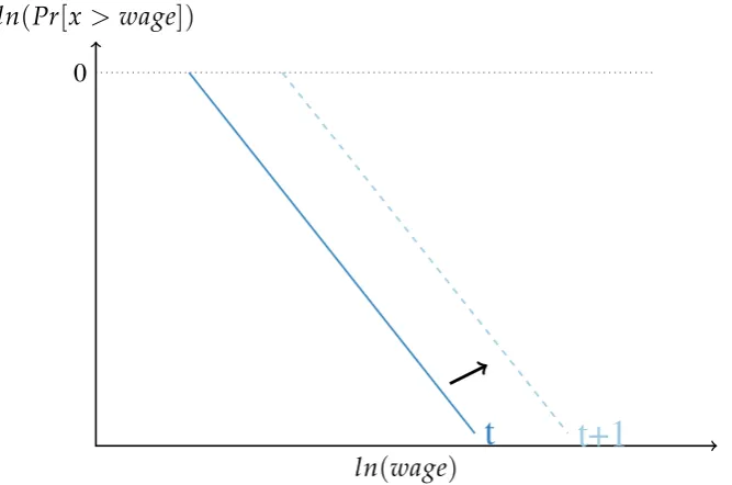
The Effect of Technical Change

The remainder of this section illustrates a pattern in wage changes that allows to distinguish the superstar channel from other potential channels. In the empirical application the exogenous instrument will rule out spurious findings from range of mechanisms, however, such exogenous variation in technology does not rule out that technical change affects wages through other channels than superstar effects. To 14_{This additional restriction is not required in other versions of the superstar model. For example,}

Sattinger(1975) assumes log super-modularity in production and does not require additional assumptions on the spacing of the distributions.

(24)

distinguish different models of technical change, I derive patterns of wage changes from the superstar model that are distinct from conventional models of technical change.

2.2.1 Superstar Effects and Technical Change

The superstar effect is the result of expanding markets reach. A tractable way of modeling such a change is allowing production to become more scalable and thus reducing the diseconomies to scale in the production function. Assume that this change takes the form ofδ0 = s·δand γ0 = s·γ withs > 1.15 The new wage distribution

(call the new periodt+1) is therefore found by substitute the new valuesξ0andλ0into

equation6:

pw_t₊₁ =λ0wp

−ξ0

α (8)

Since we assumed that labor supply is inelastic we can solve for wage growth by dividing the new and old wage distributions evaluated at percentile p. Wages int+1 are given by 8 and period t wages are given by 6. Wage growth at percentile p is therefore:

gwp =

wtp+1

wt p

=ψp

−α

ξ (s−1) (9)

Where ψ = (λ 0

λ)

α(s−1)

ξ _{. These equations reveal, that the reduction of diseconomies}

to scale has differential effects at different parts of the distribution. The effect are summarized in Figure1, the wage distribution shifts inward and pivots out. The intuition is that more productive workers are matched with bigger shows and therefore operate on a bigger scale, diseconomies to scale are more binding for this group. Such top workers therefore benefit most from better scalability of production. The effect can be seen in two changes in equation 8, the shape and scale parameter of the Pareto wage distribution change. Compared to equation 6 ξ0 = ξ_s < ξ, which implies that wage

differences between workers grow, the wage distribution pivots out and the distribution becomes more right skewed. Besides this top income growth, there is an additional level effect on the wage distribution operating throughλ0. This is a level effect that reduces

wages at all levels. The level effect is a consequence of expansion in the availability of entertainment, since more entertainment is being produced, the entertainment market clears at a lower price for talent π.16 As a result the Pareto scale parameter falls

15_{An alternative but ultimately equivalent way of modeling this change is to allow the size distribution}

to change, for example by increasing the shape parameterα(see Appendix8.C).

16_{If we maintain that the outside option is fixed at a level} _b_{, the lowest wages are fixed at} _b _and

adjustment occurs through exit rather than falling wages. Wages at the bottom could decline if there is a cost to exiting, for example search costs, or if payoffs from the outside option also fall.

(25)

(λ0 <λ) and the wage distribution shifts inward (see equation8).17 This case illustrates

one of the key features of a superstar model, the potential for cannibalization effects. The greater availability of stars, reduces demand for the rest of the profession and in the limit, a single superstar serves the entire market. In summary, the bottom of the distribution benefits little from better scalability but suffer from the fall in the price for talent units, while at the top of the distribution the bigger scalability over-compensates for the fall inπ. Previously unattained income levels are reached at the top and bottom

ends of the distribution, while mid-paid jobs simultaneously disappear.

For empirical tests, it will be useful to derive separate predictions for different parts of the distribution. I will illustrate the effect of technical change by deriving which types of jobs are created and which ones are being destroyed. Consider the number of jobs that pay wagew, given by the density of the wage distribution f(w). To derive the density take the derivative of5with respect towand multiply by minus one:

f(w) = λξ

α w −ξ

α−1

The two effects of technical change are visible again here. Since ξ0 = ξ_s < ξ and λ0 < λthe Pareto scale parameters falls, while the shape parameter α_ξ increases. This

again leads to a level decrease but an outward pivot of the distribution. The implications for the growth of high and low paid jobs can be computed by dividing the mass of jobs with wagewin periodt+1with its mass in periodt. The growth in the share of actors with wagew, denoted byge(w), is given by:

ge(w) = ft+1 (w)

ft(w)

= λ

0 ξ0 λξ w

(s−1) s

ξ

α −1 (10)

This growth rate is illustrated for different wage bins in Panel B of Figure 1. While the magnitude of the changes depends on distributional assumptions, the pattern is independent of these assumption. Jobs that pay at the extremes of the distribution are becoming more common, while mid-income jobs are disappearing. The effect of technical change is therefore U-shaped across the wage distribution. To see this note that ge(w)is increasing inwand will be positive for largew. The fraction of top paid actors

is therefore growing, with effects becoming more pronounced at higherw. By contrast, for lower values ofwthe growth rate turns negative since λ0ξ0

λξ < 1. Also note that the two distributions do not have the same support. Incomes that were previously outside the range of the income distribution appear in both tails of the distribution through technical change. The growth rate of such previously non-existing job types is undefined, as we would divide by zero. However, the share of jobs increases unambiguously. Panel B of Figure1groups the wage tails into a final wage bin and report the growth rate for a bin

17_{Notice that if}

π is unchanged (ie if demand for entertainment is perfectly elastic),λwould rise. I assume that demand is sufficiently inelastic to rule this case out.

(26)

that has support in both distributions. By using wage bins I can compute growth rates for wage bins that span the full wage distribution.

2.2.2 Alternative Models of Technical Change

Next, I compare the effect of technical change in a superstar model to it’s effect in conventional models. A key difference between superstar models and standard labor demand models is worker substitutability. In a superstar model all worker types are unique and imperfectly substitutable, while in standard labor demand models some worker groups are perfectly substitutable, and this difference has testable implications for the effect of technical change. A classic case is the canonical model of “Skill Biased Technical Change” (SBTC). This model features low- and high-skill groups and workers within each skill group are perfectly substitutable. This simple model is silent on top income dispersion, but can be extended to feature a continuum of worker types. To contrast this with superstar models, I maintain perfect substitutability within skill groups but allow two workers in the same skill group to have different skill quantities. The literature refers to such differences in skill quantity as “efficiency units”. Assume workers at percentilephave an amount of skillqpwithqp ∼Q(p). Since the skill units

are perfect substitutes, the model features a single market clearing price for skillπ(this

type of model is developed inStigler(1961)).18 Workers are paid in proportion to their skillw = pq. With the right distribution of efficiency units, the SBTC model fits any wage distribution, therefore in the cross-section, the SBTC model is indistinguishable from the superstar model.

To examine the differences between the heterogenous workers who are perfect versus imperfect substitutes, I focus on a single group. Specifically, I will abstract away from the low-skill group and focus on income dispersion among the high-skilled.19 First consider the baseline case, where labor supply is perfectly inelastic and all workers with skill above p¯ are participating in the market.20 A skill-biased demand shift (SBD) increases the demand for talent D(π) to D0(π) > D(π).21 Market clearing implies

that increase in demand for talent increases the price of talentπ toπ0. A unit of talent

18_{Note that we can make the SBTC coincide with a model of unique talent. This would require that}

the number of skill groups goes to infinity; eventually each worker is her own skill group and thus is imperfectly substitutable. In that case, differences between the SBTC and superstar models are a result of the type of technical change. In the superstar model, star workers displace other workers, while in SBTC models workers of different types are q-complements.

19_{The results for the fully fledged model are equivalent and presented in Appendix}_8.C.

20_{This assumption is immaterial here but becomes relevant if one introduces matching (as in}_Eeckhout

and Kircher(2018)).

21_{In the conventional model, the demand shift is a result of a skill augmenting change in productivity}

(see Appendix8.C). Here we take the reduced form approach of modeling the skill-biased demand shift as a change in the demand for talent.

(27)

becomes more valuable, and the more talent a worker has, the more she benefits from the growth inπ. After a SBD shock in periodt+1wages at percentile pare given by:

wtp+1 =π0·qp=wtp π0

π

The effect of a skill-biased demand shift is proportional to the previous wage level. The wage growth at percentile pis given by:

gw_p = π

0_·_q p

π·qp

= gw (11)

Notice that gw does not carry a subscript for percentiles. All wage increases are proportional to talent and the growth rate is therefore constant across all percentiles. The intuition for this result is that workers are perfect substitutes. If a worker can be replaced by two workers with half the talent, wages are thus always proportional to the difference in talent. Wage growth is equal to growth in the skill premium (gπ ₌ π0

π > 0), independent of p. To compare the results to the superstar effect, assume as above that talent is Pareto distributed (p = q−1eα).

22 _{This allows us to solve for the wage}

distribution:

pt = (w/π)−

1

e

α

The growth in the skill premium toπ0leads to an outward shift in the wage distribution

that is illustrated in logs in Figure 2. First, notice that the original wage distribution is identical to the result of the superstar model. With the right assumption on its parameters, the SBTC and superstar models yield the same result and makes the two models indistinguishable in cross-sectional data.

2.2.3 Testable Differences

Technical change, however, leads to a distinctive change, visible in Figures 2 and 1. The SBTC and superstar models have strikingly different effects: the former leads to an intercept shift, while the latter shifts and pivots the wage distribution. Cannibalization effects and fractal inequality distinguish the two models from one another. Fractal inequality refers to pay growth at the top that becomes more pronounced as one moves up the top tail of the pay distribution. Cannibalization indicates that top income growth is accompanied by negative effects for mediocre workers. This is visible at the middle 22_{To cut through the debate on assumptions related to the talent distribution, I show which talent}

distribution is required for this model to match the 1939 wage distribution and what shift in the skill premium is needed to account for the growth in top earners between 1939 and 1969. The predicted wage change pattern for the rest of the distribution is shown in the Appendix Figure12.

(28)

and bottom parts of the wage distribution, where mid-income jobs disappear and low-pay jobs emerge. These effects are summarized by four testable propositions:

Proposition 2.1. Top pay growth: For two percentiles at the top of the wage distribution

p0 > pa superstar effect predicts that wage growthgw meets: gw_p0 >gw_p , while a SBD

shock hasgw_p0 =gw_p.

A superstar model generates disproportionate gains at the top, while wages grow proportionally to the level of skill in a model of SBD shocks. The SBD model does not generate skewed income growth because of the law of one price. The shift in the price for talent will affect all talent units equally and therefore lead to wage growth that is proportional to a worker’s talent. As a result, the wage growth rates are the same across the distribution.23 The result follows immediately from equations9and11.

Proposition 2.2. Mediocre worker pay: In a superstar modelwt_p+1 < wt_p is feasible,

while in a SBD modelwt_p+1 >wt_pat all percentiles.

Mediocre workers lose out due to superstar effects, while wage growth is always positive in the SBD model. A SBD shock is a positive demand shift that increases wages across the board. The first part of the proposition follows straight from equation

11. For the second part, consider equation 8and solve for the wage: wtp+1 = (λ 0

p) α ξ0

. Technical progress leads to negative wage growth ifλdeclines fast enough. To see this

let p →1, wages at the bottom of the distribution converge towtp+1 → (λ0) α ξ0

. Falling wages occur if(λ0)

α ξ0

< (λ) α ξ

, or if demand is sufficiently elastic. The intuition is that in the superstar model, technical progress allows stars to steal some of the business of lesser stars, while in the SBD model q-complementarity of worker types guarantees that wages grow if any type becomes more productive.

Proposition 2.3. Employment: In a superstar model p¯t+1 > p¯t, while in a SBD model ¯

pt+1 < p¯t.

With entry and exit, the participation thresholdp¯determines which worker are active in the market. Employment declines in a superstar model as stars’ growing reach pushes other workers out of the market. With positive demand shocks, by contrast, quantity and wages move in the same direction. The price for talentπrises in response to SBD

shocks but falls with superstar effects. The proposition then follows from the market clearing condition in equation25, meaning that a higher price for talent leads to more participation.

Next I focus on dispersion in top incomes and focus on the predicted change in top income shares.

23_{With additional skill groups this holds approximately for the highly talented individuals within a skill}

group.

(29)

Proposition 2.4. Dispersion at the top: Income differences within the top tail increase

with superstar effects but not with SBD shocks. This implies for top income shares (sp)

at two percentiles p: st_1%+1/st_10%+1 > s_1%t /s_10%t in a superstar model and st_1%+1/st_10%+1 =

s_1%t /st_10%in a SBD model.

This proposition highlights the income dispersion within the top tail. A superstar model exhibits a fractal inequality, so that moving up a rank in the talent distribution becomes more valuable. As a result, a growing proportion of the the income share of the top 10% is earned by the top 1% and consequently the ratio of the two (s1%/s10% ↑)

increases. The same increase in fractal inequality does not hold in the SBTC model, where the relative pay differences remain stable. The proposition is derived in Appendix

8.C.

A natural question is whether extensions to the SBTC model allow it to replicate these results. The key distinction highlighted so far is that a SBTC model features groups of perfectly substitutable workers, whereas workers are imperfect substitutes in the superstar model. However, there are additional differences between superstar and SBTC models. To see this, consider the case where there is a continuum of skill groups in the SBTC model. Workers in two different skill groups are imperfect substitutes, with a continuum of skill groups each worker is his own skill group and hence all workers are imperfect substitutes. This extended SBTC model can generate fractal wage inequality, it requires technical change that increases productivity in an escalating fashion towards the top. However, the model will not feature cannibalization effects. A positive demand shock translates into gains across the range of the distribution, which is proved in Appendix 8.C. Even a SBTC model where all workers are imperfectly substitutable will therefore not feature cannibalization effects and will not replicate propositions2.2

and2.3.

In summary, the superstar effect leads to four testable predictions: 1. disproportional wage growth at the top,

2. decreasing wages for mediocre workers, 3. falling employment and

4. growing dispersion of wages at the top.

Effects one and four reflect the fractal inequality effect, while effects two and three capture the cannibalization effect.

3

Data

I collect novel data on the production and consumption of entertainment in the middle of the 20th century from archival sources. Consumption data includes local-level

(30)

consumer spending and attendance at entertainment venues, while the production data includes information on local inputs and production technology. These data are linked to entertainers’ labor market records.

3.1

Production Technology

TV Data For each labor market I compute two measures of TV: exposure to television filming and exposure to television broadcasting. The first captures the change in the production technology and records where TV shows are produced. The second measures where local entertainers face competition from television.

Television Filming Data on television facilities come from the “Annual Television Factbooks” which records the address, technical equipment, launch date, assigned channel and call letter for each TV station.24 I geocode the location of TV studios and match them to the local labor market to track the roll-out. The launch of TV filming provides one of the main sources of variation in the analysis, Figure 3 shows where broadcasting took place in the year 1949, a year with Census wage data. For each year I compute the exposure to local TV filming by summing the number of active stations in the local labor market and therefore assume that all stations were filming locally at that time. There are a handful of exceptions, as a few stations operated a local network. These interconnected stations could relay local shows to nearby stations through upgraded phone lines (run by AT&T) or microwave relay technology (run by Bell). Interconnection was rarely feasible because the technical infrastructure was still in its infancy. In my main specifications I code all members of such networks as treated. This approach avoids potential endogenous selection of filming locations within the network.25

TV Licensing Detailed information on the licensing process allows me to identify places that narrowly miss out on TV launches during the license freeze. The freeze in licenses began in 1948 and continued until 1952. The data are based on the weekly bulletins from the Federal Communication Commission (FCC), which are summarized annually in the “Television Factbook.” From the same records, I collect information on the rule used to prioritize locations. This rule was published in a few years and reveals that the priority ranking of the TV roll-out was based on fixed location characteristics. This lends credibility to the assumption of the difference in differences regression, that the TV timing did not respond to local demand shocks.

24_{This data source has previously been used by} _Gentzkow _{(2006) to build a dataset of TV signal}

coverage throughout the US.

25_{Robustness checks explore alternative treatments. As expected, within those networks effects on top}

incomes appear in the labor market where filming is mostly located.

(31)

Videotape Filming Local filming was ultimately superseded by centralized produc-tions. With the invention of the videotape in 1956 television production shifted away from local stations, towards places where conditions for filming are most favorable. Centrally produced shows could then be broadcast across the country at low cost and at the time appropriate for the local time zone. The rise of centralized filming leads to a decline of local TV filming which allows me to test whether local superstar effects disappear.26 To do so, I will control for places where filming centralizes, which raises the potential challenge of an endogenous control variable. To avoid this endogeneity issue, I proxy locations of centralized filming with locations where movie filming took place in the 1920s. This measure is pre-determined and picks up location incentives that come from permanent regional characteristics. The data on the location of film shoots come from the “Internet and Movie Database” (ImDB). ImDB is a widely used platform (self-proclaimed number one worldwide) for information on movies and holds metadata on over 4 million movies. In 1920, around 200 movies were produced in the US. For each labor market I compute the share of movies produced in this market in 1920.

3.2

Demand Data

Television Broadcasting Data on TV signal allows me to establish when local entertainer start facing competition from TV entertainment. Places that are exposed to TV signal are not necessarily the same as labor markets that produce TV shows, as signal airwaves travels beyond the local labor market of the TV station. Information on TV stations’ signal reach comes fromFenton and Koenig(2018), who re-construct historic catchment areas.27 Figure 4 shows the variation in TV signal in 1950 and illustrates areas that narrowly miss out on TV signal due to the freeze in licensing. I combine the information on each TV station’s catchment area with Census data on household location and TV ownership and compute the audience of TV shows. The median TV station could reach approximately 75,000 households. Even the smallest TV audiences substantially exceeded the show audiences of local venues.28 Additionally, I compute 26_{The invention of the videotape is another example of a technology that expanded market reach.}

However, this variation is less suitable for a test of the superstar model, the location of filming for videotape is not exogenously imposed. Instead markets with the lowest production cost were selected for filming. Production cost are determined by endogenous factors such as local wages and tax rates as well as fixed location characteristics (e.g. sunshine hours, availability of equipment and expertise, local scenery).

27_{For details on the data construction see}_{Fenton and Koenig}_{(2018). They use an irregular terrain}

model (ITM) to calculate signal propagation. In this model, signal reach depends on the technical properties of an antenna (channel, frequency, height, etc.) and on terrain that blocks airwave travel (e.g. mountains). The ITM has also been used in a number of other studies (Olken(2009);Enikolopov et al. (2011);Durante et al.(2015))

28_{For the US, alte}