A Reliable Method of Minimum Zone Evaluation of
Cylindricity and Conicity from Coordinate
Measurement Data
Xiangchao Zhang, Xiangqian Jiang∗, and Paul J. Scott Centre for Precision Technologies, University of Huddersfield, Huddersfield,
HD1 3DH, UK
Abstract
The form error evaluation of cylinders and cones is very important in pre-cision coordinate metrology. The solution of the traditional least squares technique is prone to over-estimation, as a result unnecessary rejections may be caused. This paper proposes a reliable algorithm to calculate the mini-mum zone form errors of cylinders and cones, called a hybrid particle swarm optimization-differential evolution algorithm. The optimization is conducted in two stages, so that the program can hold a fast convergence rate, while effectively avoiding local minima. Experimental results demonstrate that the proposed algorithm can obtain very accurate and stable results for the calculation of cylindricity and conicity.
Keywords: Form error, Cylindricity, Conicity, Minimum zone, Differential evolution
2000 MSC: 90C47, 90C31, 65K10
1. Introduction
The evaluation of cylindricity and conicity is among the most impor-tant problems in computational metrology because cylindrical and conical shapes are ubiquitous in precision components. Most current commercial software evaluates the form errors of cylinders and cones using the least
squares method due to its ease of implementation and the unbiasedness of its solution for uncorrelated normally distributed noise [1]. But it is likely to overestimate the form tolerance and lead to unnecessary rejections, therefore its solution is only an approximate one, rather than the optimum. Accord-ing to ISO 1101 [2], a geometrical tolerance applied to a feature defines the tolerance zone within which that feature shall be contained. This means the cylindricity tolerance is a permissible deviation zone bounded by two coaxial cylinders within which the measured data must lie in between. Similarly, the conicity tolerance is a permissible deviation zone bounded by two coaxial cones. They are minimax problems and not continuously differentiable, thus very difficult to be solved.
A lot of linear programming techniques have been employed for the eval-uation of straightness and flatness, e.g. simplex method [3], data exchange algorithm [4] and support vector machine [5]. The calculations of roundness and sphericity are quadratic programming problems. [3] and [6] approxi-mately linearized the formulation and solved it using the simplex technique. Computational geometry methods were also utilized to calculate flatness [7] and sphericity [8, 9]. Venkaiah and Shunmugam calculated cylindricity by identifying ‘extreme points’ to form a limacon-cylinder [10]. These meth-ods are developed for a particular shape. So far no computational geometry method has been found in literature for evaluating conicity. Recently Huang and Lee solved the conicity problem using minimum potential energy algo-rithms [11], which are very elaborate. Some researchers attempted to ap-proximate the cylinder/cone iteratively and then solved a sequence of linear programs [12, 13], but these methods need a very good initial guess and are prone to sub-optimal solutions. Lai and Chen [14] converted a cylinder into a plane and obtained appropriate control points. The cylindricity is calculated by implementing a series of inverse transformations.
In recent years heuristic search optimizers have been employed to solve the minimum zone problem. Lai et al. [15] and Liu et al. [16] used genetic algorithms to evaluate the cylindricity and conicity errors, respectively, while Wen and Song adopted an immune evolutionary algorithm for sphericity [17]. The particle swarm optimization technique was utilized by [18, 19]. The advantages and shortcomings of these algorithms will be discussed in Section 3.
accuracy, and makes a good balance between exploration and exploitation.
2. Formulation of cylindricity and conicity errors
2.1. Cylindricity error
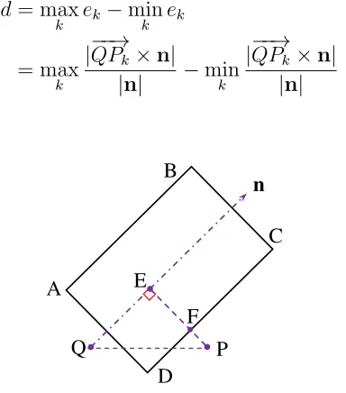
Fig.1 illustrates the cross section of a cylinder with axis directionn(m, n,1) and a radius R. The projection of a measured point P onto the cylinder is
F. Assuming the axis passes the point Q(x0, y0,0), then the axis function is (x−x0)/m= (y−y0)/n=z. The distance from P to the cylinder is,
e=|F P|=|EP| − |EF|= |
−→
QP ×n|
|n| −R
In the equation | · |means the length of a vector in the Euclidean space. Given a point setP={Pk|k= 1,2, . . . , M}, the cylindricity error is,
d= max
k ek−mink ek
= max k
|−−→QPk×n|
|n| −mink
|−−→QPk×n|
|n| (1)
n
A
B
C
D E
F
[image:3.612.211.403.356.574.2]P Q
2.2. Conicity error
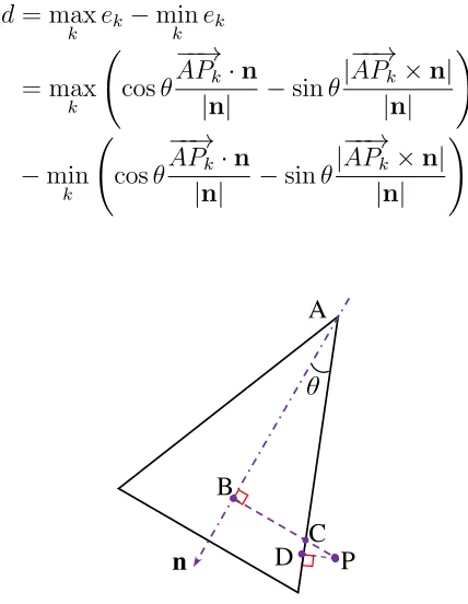
Fig. 2 shows the cross section of a cone with vertex angle 2θ, axis direction n(m, n,−1) and vertex A(x0, y0, z0). The projection point of a measured point P onto the cone isD. The distance from P to the cone is,
e=|DP|= cosθ(|BP| − |BC|) = cosθ|BP| −sinθ|AB|
Given a point setP={Pk|k= 1,2, . . . , M}, the conicity error is,
d= max
k ek−mink ek
= max k
(
cosθ
−−→
APk·n
|n| −sinθ
|−−→APk×n|
|n|
)
−min
k
(
cosθ
−−→
APk·n
|n| −sinθ
|−−→APk×n|
|n|
)
(2)
D B
A
C P ș
[image:4.612.196.410.253.529.2]n
Figure 2: Calculation of conicity error
3. A hybrid particle swarm optimization-differential evolution al-gorithm
3.1. Particle swarm optimization
In PSO, each individual, namedparticle, of the population, calledswarm, ad-justs its trajectory toward its own previous best position, and toward the pre-vious best position attained by any member of its topological neighbourhood. As a stochastic search scheme, PSO has properties of simple computation and rapid convergence capability. The individuals in evolutionary algorithms are primarily competitive. On the contrary, PSO adopts a more cooperative way. As a consequence it can find the optimal region of the solution very easily, i.e. it has outstanding capability of exploitation. Its populations move as a whole but do not evolve, thus no mutation or crossover is needed.
Suppose the search space isD-dimensional, and the positions of particles Y = {yi|i = 1,· · ·, N} are initialized using a uniform distribution. The velocity (the position change per generation) of yi at the k-th generation is given as,
vki =vik−1+c1r1⊗(pi−yi) +c2r2⊗(pg−yi), k > 1
where c1 and c2 are acceleration coefficients regulating the relative velocities toward local best pi (exploration) and global best pg(exploitation), respec-tively. r1 and r2 areD-dimensional random vectors uniformly distributed in [0,1] and⊗ denotes element-wise multiplication.
To endure convergence and to improve the stability of the basic PSO, Clerc proposed the use of a constriction factor to the velocity [21],
vik=χ[vik−1 +c1r1⊗(pi−yi) +c2r2⊗(pg−yi)], k >1 (3) Following [21], the coefficients are set as c1 =c2 = 2.05 and χ= 0.7298. Besides, a maximal allowable velocity vector Vmax is used to clamp ve-locities of particles on each dimension,
vij =
−Vmax
j vij <−Vjmax
vij −Vjmax ≤vij ≤Vjmax
Vmax
j vij ≥Vjmax
(4)
here j denotes thej-th dimension of the vector. Vmax is set according to the range of the variable space,
Vmax =γ(yU −yL)
is problem dependent. To improve the flexibility of the program, Vmax is initially set usingγ = 0.5 and then updated according to the actual situation of the running program [22],
Vmax ⇐
{
βVmax if solution stagnates for 3 generations
Vmax otherwise (5)
here β is set to be 0.95.
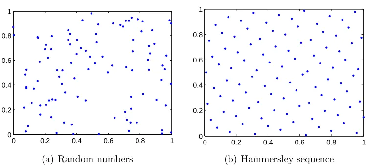
The basic PSO initializes particles using uniform pseudo-random numbers within the variable space. The random number sequences do not achieve the lowest possible discrepancy, thus the random points cannot evenly cover the whole space, as illustrated in Fig. 3(a). The discrepancy is used to mea-sure how uniformly distributed the point set is. Various low discrepancy se-quences have been proposed. Among them, the Hammersley sequence shows remarkable superiority on ease of implementation [23]. Thus it is adopted to generate initial particles.
Each nonnegative integer i can be expanded by a prime basep,
i=a0+a1p+a2p2+· · ·+arpr
with 0≤aj < p, j= 1,2,· · · , r. A function Φp is defined for ias,
Φp(i) = r
∑
j=0
aj
pj+1
It can be proved that for anyi≥0 andp≥2, the inequality 0≤Φp(i)<1 always holds true.
A series of prime numbersp1 < p2 <· · ·< pD−1 determine a sequence of functions {Φp1,Φp2,· · · ,ΦpD−1}. Then a D−dimensional Hammersley point
is defined as,
(
i
N,Φp1(i),· · · ,ΦpD−1(i)
)
, i= 1,2,· · · , N
0 0.2 0.4 0.6 0.8 1 0
0.2 0.4 0.6 0.8 1
(a) Random numbers
0 0.2 0.4 0.6 0.8 1 0
0.2 0.4 0.6 0.8 1
[image:7.612.118.492.124.293.2](b) Hammersley sequence
Figure 3: Uniform points generated by random numbers and Hammersley sequence
3.2. Differential evolution
Inspired by the natural evolution of biological species, Holland proposed a popular algorithm called the genetic algorithm (GA) [24]. In 1995, Price and Storn replaced the classical crossover and mutation operators in genetic algorithms by a differential operator, which leads to an algorithm called
differential evolution (DE) [25]. Compared to GA, DE is more simple but performs better on many numerical optimization problems [25]. Compared to PSO, it can cover the variable space more sufficiently and has greater probability to find the global optimum, i.e. it possesses superior capability of exploration.
At each generation, a Donor vector vi is generated for each individual of the population (called genome or chromosome) {yi|i = 1,· · · , N}. It is the method of creating this Donor vector that demarcates between various DE schemes. Two mutation schemes ‘DE/rand/1/bin’ and ‘DE/current to best/2/bin’ are applied [26] here,
vi =
{
yr+F(ys−yt) rand[0,1]< p yi+F(pg−yi) +F(yr−ys) otherwise
(6)
wherer, sandtare integers randomly selected from the range [1, N] (exclud-ing i). F ∈[0,2] is used to scale the differential vector.
demon-strates good diversity while ‘DE/current to best/2/bin’ shows good conver-gence property. Here p∈[0,1) is a user-set parameter.
After the mutation phase, a ‘binomial’ crossover operation is applied,
uij =
{
vij if randj[0,1]≤CR or j =jrand
yij otherwise
(7)
where CR ∈ [0,1) is a user-specified crossover constant and jrand is a ran-domly chosen integer within the range [1, N] to ensure that the trial vector ui will differ from yi by at least one component. The subscript j refers to the j-th dimension. rand[0,1] is a random number uniformly generated in the interval [0,1].
Then a selection operation follows,
yik+1 =
{
uk
i if f(uki)< f(yki)
yki otherwise (8)
with k and k+ 1 denoting the individuals at thek-th and (k+ 1)-th genera-tions, respectively, and f representing the fitness (here it is the cylindricity or conicity error).
The optimal configuration, i.e. the values of F, CR and p, is problem-dependent. To obtain relatively good performance in different situations, a self-adaptive DE is employed [27]. The parameters are trained through the optimization process. The training procedure will not be presented here for the sake of concision.
3.3. A two-stage optimization algorithm
The PSO program possesses an advantage of fast convergence, but it has a tendency of premature convergence because of the possibility of over-whelming, i.e. sub-optimal groups best influence early in the search. While DE can maintain a greater diversity in the population and the individuals can travel more amply within the variable space, thus the local minimum problem can be overcome more effectively. However DE updates the individ-uals somehow ‘blindly’ and finds the optimal region more slowly than PSO. Therefore a two-stage approach is used: first search for the optimal region using PSO and then refine the solution by DE. The criterion adopted for switching between these two stages is the diversity, which is defined as [28]
diversity(Y) = 1
N·L
N
∑
i=1
v u u t∑D
j=1
where y = ∑Ni=1yi/N is the centroid of population and L is the length of the diagonal in the search space.
The pseudocode for the two-stage optimization program is shown in Al-gorithm 1.
3.4. Implementation issues
It is obvious that Eq. (1) has only four independent variables {x0, y0,
m, n} whereas the nominal radius R can vary arbitrarily without altering the cylindricity error. The reason is only the difference between maxkek and minkek is used but their own values are not taken into account. In prac-tice, the valueα = maxkek/minkek will be supplied in different situations of surface mating. In this paper we enforce the tolerances are symmetric, i.e.
α = −1. As a result the individuals in the program need only four dimen-sions, rather than five. The radius is enforced R = 0 during optimization and then adjusted as,
R⇐ maxkek+ minkek
2
For the same reason, the conicity program has only five independent variables, rather than six. The vertex position of the nominal cone cannot be determined through the optimization program. To eliminate the ambiguity in the solution, the vertex is forced located on theX−Y plane,i.e. z0 = 0 during optimization and then worked out after that. For symmetric tolerances,
x0 ⇐x0− m(max2k|nek|sinθ+minkek)
y0 ⇐y0 −
n(maxkek+minkek)
2|n|sinθ
z0 ⇐ −maxk2e|nk|+minsinθkek
4. Experimental validation and discussion
To validate the proposed algorithm, four benchmark data sets are used. They are two cylinders from [12] (dataset 2) and [15], and two cones from [16] and [29]. Many researchers compared their own calculation results using these data. The best fitting results found in literature are presented in Table 1.
Input: X
// data points
Initialize populationY ∈RN×D, velocitiesV ∈RN×D andVmax ∈RD;
k= 0; // generation number for PSO
while k < k1max do
k+ +;
for i= 1 to N do Evaluate f(yi);
Update pi and pg if possible; Adapt vi with (3) and (4); yi ⇐yi+vi;
end
UpdateVmax with (5); if diversity(Y)< d0 then
Break; end
end
InitializeF, CR and p;
k= 0 // generation number for DE
while k < k2max do
k+ +;
Train F, CR and p; for i= 1 to N do
Mutation and crossover of yi with (6) and (7); Selection of yi with (8);
end
if termination condition satisfied then Break;
end end
Output: pg
particles was N = 20. The fitness value associated with the global optimal solution pg at every generation was stored. If the program stagnates for 30 iterations, i.e. f(pkg)−f(pk+30g ) < ϵ, the program will be terminated. Here it is set ϵ= 10−6.
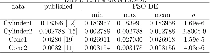
The program was run 400 times and the minimal, maximal and mean values of the cylindricity errors are listed in Table 1. The standard deviation
σof the 400 errors is applied to measure the uncertainty. It is directly related with the stability of the program. The optimal solutions obtained via this PSO-DE algorithm are listed in Table 2.
It can be seen that the program can find better results than the cited papers. It behaves very stably for the second cylinder and the global optimal solution can always be found. On the contrary, the uncertainty of the first cylinder is a little greater. This is because there are only 20 data points and the data range in the z direction is only a third of the cylinder radius, which makes the evaluation program less stable. But the relative uncertainty of the cylindricity is 0.0000092, which is sufficient for practical applications. In fact, by altering the termination conditions and increasing the particle population, the individuals can search more sufficiently within the variable space and the solution can be made more stable, of course, with a cost of more computation time.
[image:11.612.124.487.539.632.2]It has to be mentioned that [19] gave form errors 0.174635 and 0.002788 for cylinders 1 and 2, respectively. They introduced a vertex angle in the optimization program, which in turn added one extra degree of freedom in the variable space. Consequently the form errors they gave were actually conicity, rather than ‘cylindricity’. The result of cylinder 2 appears correct. It is because the vertex angle is very small, which by chance has little influence on the evaluation result.
Table 1: Form errors of PSO-DE
data published PSO-DE
min max mean σ
Cylinder1 0.18396 [12] 0.183957 0.183991 0.183958 1.69e-6 Cylinder2 0.002788 [15] 0.002788 0.002788 0.002788 2.800e-9
Cone1 0.0280 [19] 0.026911 0.027030 0.026918 1.59e-5 Cone2 0.0032 [11] 0.003154 0.003178 0.003156 4.03e-6
Table 2: Best solutions of PSO-DE to cylinders
data x0 y0 m n R
[image:12.612.114.506.219.265.2]Cylinder1 0.010650 0.046918 -0.000619 -0.002915 59.989505 Cylinder2 0.003390 -0.008381 -0.013961 0.007043 12.001374
Table 3: Best solutions of PSO-DE to cones
data x0 y0 z0 m n θ
Cone1 22.249169 10.087816 -15.768426 9.874e-3 2.337e-3 0.240671 Cone2 8.806048 3.989779 -6.169093 1.497e-3 -5.96e-4 0.239001
as well as standard deviation of 400 results are given in Table 1 and the optimal solutions are shown in Table 3. The superiority of this algorithm is more remarkable for cones. Even the worst results are better than the cited papers. This means those algorithms were trapped at local minima. Another point worth noting is that the vertices of both two cones are above the point sets, so that it is proper to set the direction vector of the axis to be (m, n,−1). If vertices are below, the direction vectors should be (m, n,1) accordingly, or equivalently make the half vertex angle −π/2 < θ < 0. In fact, to make the optimization program more flexible, the variation range of the angle can be set as −π/2 < θ < π/2, which needs no prior information on the orientation of the cone.
To reveal the behaviour of the algorithm more sufficiently, Two parame-ters y0 and n of cylinder 2 were fixed at the optimal solution, and only the other two parameters x0 and m were altered, as illustrated in Fig. 4(a) and 4(b). The gray background represents the values of the objective function associated with different (x0, m). The error map is not smooth. Instead, it contains many ‘grooves’, which imply local minima. Randomly generating 10 particles in the variable space, Fig. 4(a) and 4(b) illustrate the trajectories of the 10 particles during PSO and DE optimization, respectively. The ‘stars’ in the graphs denote the global optimal solutions.
To demonstrate the reliability of the proposed PSO-DE algorithm clearly, the variable range was set very large. In fact, the measured data can be fitted first with linear least squares [30], so that an approximate solution is obtained. Then the search space of the PSO-DE program can be greatly reduced and the computational efficiency will be improved significantly.
5. Conclusions
This paper presents a reliable method to evaluate the minimum zone form errors of cylinders and cones, which are consistent with the definitions in ISO 1101. A hybrid particle swarm optimization-differential evolution algorithm is proposed, which conducts optimization in two phases. Taking its advan-tage of fast convergence, particle swarm optimization is firstly implemented from a very large variable space. Then differential evolution is employed to search the optimal region amply, so that local minima can be effectively avoided. To improve the flexibility of the optimization program, the control parameters, e.g. the crossover rate, are trained using a self-adaptive ap-proach. Experimental examples show that this algorithm can achieve higher evaluation accuracy, and obtain better results than literature. It is versa-tile and can be extended to the minimum zone evaluation of more complex shapes, e.g. ellipsoid, paraboloid and freeform surfaces. Moreover the eval-uation criteria can also be minimum circumscribed features or maximum inscribed features, which are suited for different functionality requirements [3, 31]. Therefore, this method could be used for online inspection in high precision manufacturing or form error evaluation on coordinate measuring machines.
Acknowledgements
The authors gratefully acknowledge the Royal Society for a Wolfson Re-search Merit Award and the European ReRe-search Council for its programme ERC-2008-AdG 228117-Surfund.
References
[2] ISO 1101 . Geometrical product specifications-geometrical tolerancing-tolerances of form, orientation, location and run-out. 2004.
[3] Chetwynd DG. Applications of linear programming to engineering metrology. Proceedings of the Institution of Mechanical Engineers 1985;199(B2):93–100.
[4] Huang ST, Fan KC, Wu JH. A new minimum zone method for evaluating straightness errors. Precis Eng 1993;15(3):158–65.
[5] Malyscheff AM, Trafalis TB, Raman S. From support vector machine learning to the determination of the minimum enclosing zone. Comput-ers and Industrial Engingeering 2002;42(1):59–74.
[6] Kanada T. Evaluation of spherical form errors: computation of spheric-ity by means of minimum zone method and some examinations with using simulated data. Precis Eng 1995;17(4):281–9.
[7] Lee MK. A new convex-hull based approach to evaluating flatness tol-erance. Comput Aided Des 1997;29(12):861–8.
[8] Huang J. An exact minimum zone solution for sphericity evaluation. Comput Aided Des 1999;31(13):845–53.
[9] Samuel GL, Shunmugam MS. Evaluation of sphericity error from form data using computational geometric techniques. Int J Mach Tools Man-ufact 2002;42(3):405–16.
[10] Venkaiah N, Shunmugam MS. Evaluation of form data using computa-tional geometric techniques-part ii:cylindricity error. Int J Mach Tools Manufact 2007;47(7-8):1237–45.
[11] Huang PH, Lee JC. Minimum zone evaluation of conicity error using minimum potential energy algorithms. Precis Eng 2010;34(4):709–17.
[12] Carr K, Ferreira P. Verification of form tolerances part ii: cylindricity and straightness of a median line. Precis Eng 1995;17(2):144–56.
[14] Lai JY, Chen IH. Minimum zone evaluation of circles and cylinders. Int J Mach Tools Manufact 1996;36(4):435–51.
[15] Lai HY, Jywe WY, Chen CK, Liu CH. Precision modeling of form errors for cylindricity evaluation using genetic algorithms. Precis Eng 2000;24(4):310–9.
[16] Liu CH, Jywe WY, Chen CK. Quality assessment on a conical taper part based on the minimum zone definition using genetic algorithms. Int J Mach Tools Manufact 2004;44(2-3):183–90.
[17] Wen X, Song A. An immune evolutionary algorithm for sphericity error evaluation. Int J Mach Tools Manufact 2004;44(10):1077–84.
[18] Kowur Y, Ramaswami H, Anand RB, Anand S. Minimum-zone form tolerance evaluation using particle swarm optimisation. Int J Intelligent Systems Technol Appl 2008;4(1-2):79–96.
[19] Wen XL, Huang JC, Sheng DH, Wang FL. Conicity and cylindric-ity error evaluation using particle swarm optimization. Precis Eng 2010;34(2):338–44.
[20] Kennedy J, Eberhart RC. Particle swarm optimization. In: Proc. IEEE Int. Conf. Neural Networks; vol. 4. Perth, Australia; 1995, p. 1942–8.
[21] Clerc M, Kennedy J. The particle swarm-explosion, stability and conver-gence in a multidimensional complex space. IEEE Trans Evolut Comput 2002;6(1):58–73.
[22] Fourie PC, Groenwold AA. The particle swarm optimization algorithm in size and shape optimization. Structural and Multidisciplinary Opti-mization 2002;23(4):259–67.
[23] Wong TT, Luk WS, Heng PA. Sampling with hammersley and halton points. J Graphics Tools 1997;2(2):9–24.
[25] Price KV, Storn RM, Lampinen JA. Differential evolution: a practical approach to global optimization. Natural Computing Series; Berlin: Springer; 2005.
[26] Qin AK, Suganthan PN. Self-adaptive differential evolution algorithm for numerical optimization. In: 2005 IEEE Congress on Evolutionary Computation; vol. 2. 2005, p. 1785–91.
[27] Jia L, Gong W, Wu H. An improved self-adaptive control parameter of differential evolution for global optimization. In: Cai Z, Li Z, Kang Z, Liu Y, editors. Computational Intelligence and Intelligent Systems. Springer; 2009, p. 215–24.
[28] Ursem RK. Diversity-guided evolutionary algorithms. In: Parallel Prob-lem Solving from Nature-PPSN VII. Lecture notes in computer science; Granada, Spain: Springer; 2002, p. 462–71.
[29] Chatterjee G, Roth B. Chebyshev approximation methods for evaluating conicity. Measurement 1998;23(3):63–76.
[30] Zhang X. Freeform surface fitting for precision coordinate metrology. Ph.D. thesis; University of Huddersfield, Huddersfield, UK; 2009.
(a) PSO
[image:17.612.192.417.203.580.2](b) DE