Comparison of Type F2 Software Measurement Standards for Surface Texture

Li, T., Leach, Richard K., Jung, L, Jiang, Xiang and Blunt, Liam

Comparison of Type F2 Software Measurement Standards for Surface Texture

Original Citation

Li, T., Leach, Richard K., Jung, L, Jiang, Xiang and Blunt, Liam (2009) Comparison of Type F2 

Software Measurement Standards for Surface Texture. Technical Report. National Physical 

Laboratory, UK, London, UK. 

This version is available at http://eprints.hud.ac.uk/id/eprint/7673/

The University Repository is a digital collection of the research output of the

University, available on Open Access. Copyright and Moral Rights for the items

on this site are retained by the individual author and/or other copyright owners.

Users may access full items free of charge; copies of full text items generally

can be reproduced, displayed or performed and given to third parties in any

format or medium for personal research or study, educational or not­for­profit

purposes without prior permission or charge, provided:

•

The authors, title and full bibliographic details is credited in any copy;

•

A hyperlink and/or URL is included for the original metadata page; and

•

The content is not changed in any way.

For more information, including our policy and submission procedure, please

contact the Repository Team at: [email protected].

NPL REPORT ENG 16

Comparison of Type F2

Software Measurement

Standards for Surface

Texture

T Li, R K Leach, X Jiang and

L A Blunt

Comparison of Type F2 Software Measurement Standards

for Surface Texture

T Li

, R K Leach

, X Jiang

and L A Blunt

1.

Centre for Precision Technologies, University of Huddersfield

2.

Industry & Innovation Division, National Physical Laboratory

ABSTRACT

© Crown copyright 2009

Reproduced with the permission of the Controller of HMSO and Queen's Printer for Scotland

ISSN 1754-2987

National Physical Laboratory

Hampton Road, Teddington, Middlesex, TW11 0LW

Extracts from this report may be reproduced provided the source is acknowledged and the extract is not taken out of context.

Contents

1 Introduction...7

1.1 Background ...7

1.2 Participants and test software... 9

1.3 Scope...9

1.4 The definition of measurement uncertainty ... 10

1.5 Acknowledgements ... 11

2 Differences between national software packages...11

3 Methodology ... 12

3.1 Classification of errors and uncertainties ... 12

3.1.1 Correlation uncertainty... 12

3.1.2 Specification variation ... 13

3.1.3 Computational error ... 13

3.1.4 Data uncertainty ... 13

3.2 Evaluation of uncertainty ...13

3.2.1 Evaluation of specification variation... 14

3.2.2 Evaluation of computational errors ... 14

3.3 Decision rules and uncertainty management... 15

4 Specification of reference pairs... 16

4.1 Reference data sets...16

4.2 Reference result... 16

4.3 The performance metrics for Cos.smd ... 17

4.4 The performance metrics for measured profiles ...17

5 Specification variation ...18

5.1 Pre-process operator... 18

5.2 Levelling ...18

5.3 Evaluation length and sampling length ...18

5.3.1 R-parameters ... 18

5.3.2 P-parameters... 19

5.3.3 W-parameters ...19

5.4 Filtering... 19

5.4.1 λs filtering...19

5.5 Profile element ... 19

5.5.1 Joint direction...19

5.5.2 Incomplete portion ... 20

5.5.3 Insignificant features... 21

5.6 Discrete interpretation... 23

5.6.1 Length definition...23

Mean line crossing-points ...24

5.7 Two examples: Ra and RSm... 24

6 Evaluation and discussion ... 25

6.1 Evaluation of Cos.smd ...25

6.1.1 Effect of levelling operator ...25

6.1.2 Effect of filtering...25

6.1.3 RSm/PSm...26

6.1.4 Computational error ... 26

6.1.5 Software effect ... 27

6.1.6 Fitness for purpose ... 27

6.2 Evaluation of measured profiles... 28

7 Conclusions...30

8 Reference: ... 31

9 Appendix A: Measurement conditions... 34

10 Appendix B: Tables of the Results... 35

1 Introduction

1.1 Background

Surface metrology is often a critical part of product quality control and has a close relationship to product design and manufacture. To maintain traceability for surface measurement, widely used measurement procedures and conditions are standardised, and many material artefacts are available to calibrate the vertical and horizontal characteristics of a probing system, the probe tip condition and the ability of the instrument to measure surface texture parameters (Figure 1 and Table 1). In the last two decades, there have emerged many advanced surface characterisation techniques to enhance the “quality” of the mathematical model to represent the geometrical properties of an engineered surface, such as areal characterisation, fractal parameters and various filtering methods [1, 2]. The use of digital techniques makes it possible to implement complex mathematical models and this has led to the need for more complex standardisation and calibration procedures. The assessment of the quality of a mathematical process includes two parts: the quality of the mathematical models and algorithms, and the quality of the numerical implementation, i.e. software. Compared with variations in measured surface texture caused by the surface inhomogeneity [3], the measurement environment [4], the choice of sampling interval [3], and different data collection methods (stylus, optical, AFM[5]), the variation contributed by software might seem at first sight to be insignificant. However, without a formal validation, this consideration remains intuitive and, when challenged, a convincing response is rarely provided.

Figure 1: Surface measuring procedure, some relevant ISO standards and measurement standards1

Some related work on validation of software in surface texture can be found in the literature. In 1988, Scott introduced the concept of “the reference surface measuring instrument”, a mathematically defined conceptual surface measuring instrument to provide the reference for a

1 _{The term “controlled experiments” is defined as “the activity to recognise parameters that are}

functionally important for each application and determine their control values” [6]. Thus, the use of the measurement standards does not cover the assessment of controlled experiments.

Measurement Standards ISO Standards

ISO 11562 ISO 4288

ISO 4287 Numerical objects

- Data File

Functional Performance Numerical Results

(Parameters)

ISO 3274

Mathematic Treatment Data collection & pre-processing Engineering

Surface

Controlled Experiments

ISO 5436-2

T

ype A _Type B _Type C

T

ype D

Typ

specific instrument [7]. The checking of the algorithms for calculating parameters was proposed in calibration procedures of surface profile and areal instruments [6, 8]. Stout et al. used simulated specimens with known characteristics in the form of data files to carry out software verification [8]. Two surface parameter algorithm comparisons were undertaken by the National Institute of Standards and Technology (NIST) in the USA, and showed good agreement for most parameters and most software packages but with some disagreement for a few parameters [9, 10]. Another comparison among seventeen national metrology institutes in Europe reported large differences in some height and spacing parameters [11]. These references show that software is a primary contributor to the variation of the final results.

Type A:

Depth measurement standard

Calibration of vertical displacement

Type B: Tip condition measurement standard

Calibration of the state of tip

Type C: Spacing measurement standard

Calibration of the horizontal displacement

Type D: Roughness measurement standard

Total calibration of the instrument

(parameter Ra & Rz)

Type F: Software measurement standard http://www.ptb.de/en/org/5/51/517/rptb_web/wizard/greeting.php http://syseng.nist.gov/VSC/jsp/index.jsp http://www.npl.co.uk/server.php?show=ConWebDoc.160

Calibration of software algorithms

(filter and all parameters)

Table 1: Examples of surface texture calibration standards described by ISO 5436 [12, 13] ISO 5436-2 (2000) introduced into international standardisation the concept of software measurement standards in the form of reference data (type F1 or softgauges) and reference software (type F2) to verify surface metrology software 2 _{. Physikalisch-Technische}

Bundesanstalt (PTB) in Germany has developed reference software to test software for roughness analysis [14]. NIST has developed a surface metrology algorithm testing system to serve as master algorithms to validate surface analysis software [15]. The National Physical Laboratory (NPL) in the UK, with University of Huddersfield and Taylor Hobson, has developed software measurement standards for surface topography software assessment [16]. In this report, these reference software packages are referred to as type F2 software measurement standards because they were developed to address the same requirement defined in ISO 5436-2 (2000) and are maintained by a national measurement institute (NMI) to serve as a metrological tool. All type F2 software measurement standards (later in this report referred to as simply type F2 standards) claim to have been developed to high standards and to have been thoroughly tested. However, some initial comparisons have already shown some disagreement among these type F2 standards [15]. Therefore, there are some essential questions that need to be addressed before these type F2 standards can safely and reliably be used. Some important questions are:

1) Is it safe to ignore calibration software?

2) Do the type F2 standards qualify to be used as calibration tools?

2 _{In the context of surface texture, a software measurement standard is a metrological tool (Clause}

3) How does one make a judgement when there is discrepancy between an industrial software package and a type F2 standard, or even between two type F2 standards?

To address these questions, a comparison of the three NMI’s type F2 standards has been undertaken. Six reference data sets are used to compare the results obtained from these type F2 standards together with three widely used commercial software packages. The sources of variation, including the specification variation, computational errors and data uncertainty, are analysed.

1.2 Participants and test software

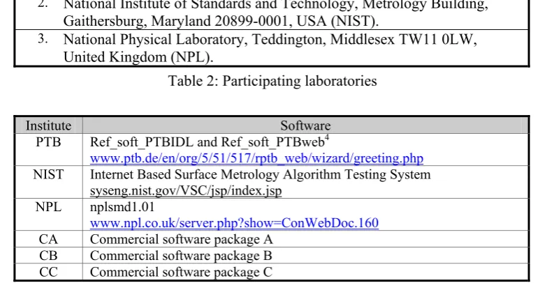
The participants in this comparison are listed in Table 2. The detailed descriptions of the type F2 standards are available online and links are provided in Table 3. In addition, three commercial software packages were used in this comparison. They are named as CA, CB and CC for commercial protection.

1. Physikalisch-Technische Bundesanstalt, Bundesallee 100, 38116 Braunschweig, Germany (PTB).

2. National Institute of Standards and Technology, Metrology Building, Gaithersburg, Maryland 20899-0001, USA (NIST).

3. National Physical Laboratory, Teddington, Middlesex TW11 0LW, United Kingdom (NPL).

Table 2: Participating laboratories

Institute Software

PTB Ref_soft_PTBIDL and Ref_soft_PTBweb4

www.ptb.de/en/org/5/51/517/rptb_web/wizard/greeting.php

NIST Internet Based Surface Metrology Algorithm Testing System syseng.nist.gov/VSC/jsp/index.jsp

NPL nplsmd1.01

www.npl.co.uk/server.php?show=ConWebDoc.160

CA Commercial software package A CB Commercial software package B CC Commercial software package C

Table 3: Type F2 standards and commercial packages

1.3 Scope

To address the major concern of metrologists, this comparison was mainly focused on the metrological traceability of the measurement results. Many software quality characteristics according to ISO/IEC 9126 [17] (i.e. usability, efficiency, maintainability, portability, etc.) have not been assessed in this report. The parameters to be compared here are those defined within ISO 4287 (1996), and the related standard documents are:

ISO 3274: 1996 and Cor 1: 1998, Geometrical Product Specifications (GPS) — Surface texture: Profile method — Nominal characteristics of contact (stylus) instruments.

ISO 4287: 1997, Cor 1: 1998 and Cor 2: 2005, Geometrical product specifications (GPS) — Surface texture: Profile method — Terms, definitions and surface texture parameters.

ISO 4288: 1996 and Cor 1: 1998, Geometrical Product Specifications (GPS) — Surface texture: Profile method — Rules and procedures for the assessment of surface texture.

3 _{The term test software used throughout this report refers to the software under test, including the type}

F2 standards and commercial packages.

ISO 11562: 1996 Cor 1: 1998, Geometrical Product Specifications (GPS) — Surface texture: Profile method — Metrological characterization of phase correct filters.

ISO 5436-1: 2000, Geometrical Product Specifications (GPS) — Surface texture: Profile method; Measurement Standards — Part 1: Material measures.

ISO 5436-2: 2000, Cor 1: 2006 and Cor 2: 2008, Geometrical Product Specifications (GPS) — Surface texture: Profile method; Measurement Standards — Part 2: Software measurement standards.

ISO 1302: 2002, Geometrical Product Specifications (GPS) — Indication of surface texture in technical product documentation.

ISO 14253-1: 1998, Geometrical Product Specifications (GPS) — Inspection by measurement of workpieces and measuring equipment — Part 1: Decision rules for proving conformance or non-conformance with specification.

ISO/IEC Guide 99: 2007, International vocabulary of metrology — Basic and general concepts and associated terms (VIM).

1.4 The definition of measurement uncertainty

Measurement uncertainty quantifies the dispersion of values attributed to a measurand. For decades, measurement uncertainty has been formulated in terms of probability theory. The most commonly used procedure for calculating measurement uncertainty is described in the Guide to the Expression of Uncertainty in Measurement (the GUM) [18]. The components of measurement uncertainty are grouped into two categories: type A and type B, according to whether they were evaluated by a statistical analysis of the values from a series of measurements or otherwise, respectively.

In the GUM, the uncertainty in communication and cognition level is considered to be negligible with respect to the other components of measurement uncertainty. However, ISO/TC 213 has recognised that the disagreement of the measurement results from two different parties is often a result of different interpretations of the specification, and/or different choices of influential conditions that are not pre-specified [19]. The concepts of method uncertainty and specification uncertainty have been introduced to quantify those uncertainties due to the “lack of information”. In ISO/TS I7450-2, the uncertainty is divided into correlation uncertainty, specification uncertainty and measurement uncertainty [20]. Measurement uncertainty includes two components, method uncertainty and implementation uncertainty. It is noted that these terms and concepts are still evolving and are subject to modification and refinement as the work of ISO/TC 213 progresses.

In VIM (2007), the concept of definitional uncertainty is introduced by ISO and IEC as a component of measurement uncertainty arising from the finite amount of detail in the definition of a measurand [21]. The definition of metrological traceabilityand measurement uncertaintyis defined as:

“Metrological Traceability: property of a measurement result whereby the result can be related to a reference through a documented unbroken chain of calibrations, each contributing to the measurement uncertainty.”

“Measurement Uncertainty: non-negative parameter characterizing the dispersion of the quantity values being attributed to a measurand, based on the information used.” (ISO/IEC VIM (2007))

According to VIM (2007), definitional uncertainty is related to the description detail of a measurand. Many description details are inside software packages. Software, therefore, is a contributor to measurement uncertainty.

1.5 Acknowledgements

The authors would like to thank the following participants in the comparison: Dr Ludger Koenders, Dr Rolf Krüger-Sehm and Dr Lena Jung (PTB), Dr Ted Vorburger and Dr Son Bui (NIST) and Prof. Paul Scott (Taylor Hobson).

2 Differences between national software packages

NIST, PTB and NPL have some differences in their interpretation of the ISO standard documents. Most of these differences are detailed in Section 5, and a summary of them is given below.

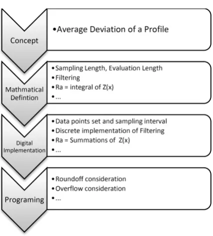
• Continuous model or discrete model: a significant difference is the type of mathematical model used to represent a surface in the ISO standard documents. Should this be a continuous model or a discrete model? Figure 2 shows the phases of applying the ISO standard documents a software implementation with the example of the Ra

parameter. The measurement procedure and condition are standardised. Some calculation phases are described clearly in mathematical models (for example, the parameter Ra); some are introduced as concepts (for example, discrimination of a profile element); while others are provided in the discrete form directly (for example, the parameter Rdq). ASME B46 provides both analytical and digital definitions [22]. PTB and NIST use a discrete model while NPL uses a continuous model.

• P-parameters and W-parameters: ISO 5436 (1996) introduces P-parameters and W -parameters into ISO standards. There are differences about the sampling length of P -parameters and W-parameters (see Section 5.3).

• Levelling:there is a difference about the levelling operator (see Section 5.2).

• RSm/PSm/Pc/Rc parameters: the interpretations of these parameters vary among NIST, NPL and PTB. This is because the definition of a profile element is ambiguous in ISO 5436 (see Section 5.5).

• SMD format:ISO 5436-2 introduces the SMD file format as the protocol of software calibration. However, different interpretations of the SMD file format are provided by NPL and PTB [11].

This report discusses the measurement conditions and parameter specifications mainly based on

Figure 2: Phases of applying the ISO standards

3 Methodology

3.1 Classification of errors and uncertainties

In VIM (2007), the concept of measurement uncertainty is extended to cover definitional uncertainty. The current versions of the GUM and ISO/TS 17450 are based on the previous definition of measurement uncertainty. There is no guidance on how to express and estimate the definitional uncertainty5_{. In this report, we combine the concepts from the GUM and ISO/TS}

17450 to describe the sources of errors and uncertainties from a software perspective. The variation in the final results obtained from different software comes from a variety of sources (see Figure 3) and is discussed below.

Figure 3: Sources of error and uncertainty

3.1.1 Correlation uncertainty

The correlation uncertainty is defined within ISO/TS 17450 as the difference between a functional requirement and an actual geometric specification. Correlation uncertainty varies from application to application and should be evaluated by experiment. Thus, software measurement standards do not take correlation uncertainty into consideration.

5 _{The VIM(2007) does not define the concept of measurand definition, while it is still an open topic in}

the field of metrology [24-28].

Computer Model Mathematical

Model Surface

Numerical Results Input Data

Data Uncertainty

Specification Variation Correlation Uncertainty

3.1.2 Specification variation

To develop surface metrology software, a full mathematical specification is required. The term specification variation is used to describe the variation of the full mathematical specification between different software packages6_{. The main sources of specification variation are listed}

below.

1. Incomplete definition in an ISO standard. For the ISO standards documents, it is impossible and unnecessary to detail every measurement procedure and condition because standards need to achieve a balance between over-specification and lack of focus. Incompleteness of the definition can lead to ambiguity and implementation in different ways by different software developers based on their own knowledge and experience.

2. Imperfect definition in an ISO standard. We may never claim perfection in standards because the standards development process is in a continuous improvement mode7_.

Instrument manufacturers may adhere to the definitions or make an improvement. 3. The transformation between different models. Generally, the conceptual model and

mathematical model are based on a continuous profile, while the implementation model is based on a discrete profile. There are errors and uncertainties when mapping one model to another.

4. Mistakes. There are human errors due to the misinterpretation and misunderstanding of ISO standards.

Many specification variations are negligible with respect to the other components of measurement uncertainty. For software validation, the main tasks are to evaluate the effect of the influencing conditions which are not standardised, and that of significant mistakes.

3.1.3 Computational error

A well-known source of error is contributed by the limitation of the computer. Due to the computer’s binary representation of numbers with finite precision, there are two types of errors when engaging in numerical computation: rounding error and truncation error that are contributed by the computer hardware and software separately [29]. Another source of inaccuracy is the numerical algorithm itself. There can exist many different ways to compute a quantity, and some are better than others. Such errors are referred to as computational errors in this report.

3.1.4 Data uncertainty

In addition to the above, there are errors within the input data (the measurement data) due to noise, variation of the measurement environment, etc. These errors are referred as data uncertainty in this report. Investigating and quantifying such data uncertainty is the subject of uncertainty evaluation (GUM), based on a statistical model.

3.2 Evaluation of uncertainty

The evaluation of the data uncertainty would require knowledge of the uncertainties associated with the measured co-ordinates of the points. The type F2 standards of NPL and PTB do not provide the (measurement) uncertainties associated with the calculated reference values for the surface texture parameters. NIST’s type F2 standards evaluate the uncertainty due to data uncertainty using Monte Carlo simulation (MCS) [15]. NIST simulates the measurement error

6 _{We do not use the term “specification uncertainty” (defined in ISO/TS 17450-2) due to 1) specification}

uncertainty is used to quantify the communication uncertainty between designers and metrologists; 2) it is difficult to distinguish between the specification uncertainty, method uncertainty and implementation uncertainty in surface texture measurement.

7 _{However, we could say that the standards are based on the best knowledge for surface texture at the}

by adding normal distributed random noise to the co-ordinates of each data point. In this comparison, MCS will be used to estimate the contribution of data uncertainty to the final results.

Due to the fact that software packages often do not disclose detailed information of the algorithm or methods of implementation used, the full specification is normally not readily apparent from documents within the software packages. Therefore, a comparison of output of the different software packages for the same input - black box testing - is the preferred method used in the testing of software implementations.

3.2.1 Evaluation of specification variation

The specification variation is generally fixed within a particular application. Thus, we evaluate it by a testing procedure that is divided into the following stages:

1. identifying the influential conditions which are ambiguous, 2. listing all possible interpretations of those conditions, 3. estimating the effect on the final results.

In stage 1, we use two methods to identify the source of specification variation, a) the top-down method, by analysing the definition given by ISO standards, and b) the reversing method, by analysing the unexpected variation of the final results obtained from test software.

In stage 2, the possible interpretations are listed by reviewing the existed publications, and available documents of software packages.

In stage 3, the effect on the final results is estimated using mathematically synthesised profiles and measured profiles. Measurement profiles could be used as the reference data for purposes as follows:

• To demonstrate reproducibility of a surface measurement from a software perspective; and it also shows the stability and robustness of a parameter definition from an ISO standards perspective;

• To estimate the contribution of variation from a software perspective in the final results by comparing with the contribution from data uncertainty.

• To evaluate the robustness of a software algorithm in practice by transforming or changing measured data.

3.2.2 Evaluation of computational errors

Another key issue that needs to be addressed is the “true” value of measurement results of the reference data sets. In a mathematically well-defined model, this can be achieved by using both a high precision processor and data. NIST implements this method to produce the Statistical Reference Datasets (StRD) to benchmark statistical software packages [30]. The reference results were obtained from a multiple precision FORTRAN pre-processor and reference data sets with 500 decimal digits of accuracy. It has been used to benchmark many well-known statistical software packages such as Microsoft Excel (version: 97, 2000, XP, 2003, 2007) [31-34]. Another method is to start with some reference results and produce the corresponding reference data set by a data generator through the null-space approach [35]. NPL has implemented this approach to test a range of software packages [36, 37]. These methods are too advanced and not suitable for this comparison due to the following:

• The methods are developed for investigating the fitness for purpose of a software implementation of an algorithm to solve a specified, and well-defined, mathematical model. Unfortunately, there are significant variations in mathematical models among surface metrology software.

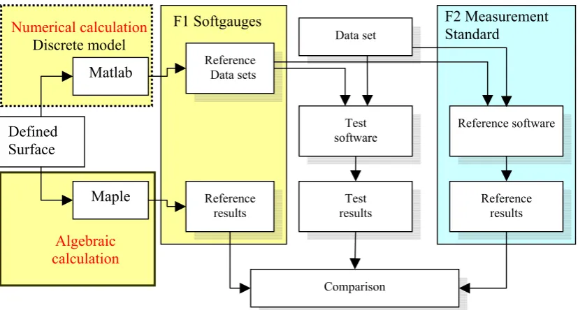
In this comparison, we use a simplified method to produce the reference pair, the reference data set and corresponding “true” result, as illustrated in Figure 4. This method uses mathematically designed synthetic reference data, by sampling mathematically defined functions for which the profile parameter values are know a priori, whose certified results can be calculated directly. This approach has the following advantages:

• The basic profile, such as a sinusoidal profile, represents the fundamental concept of the mathematical treatment for a surface profile. A reference pair is based on an unambiguous concept and mathematical model (which should be stated and agreed) with the smallest specification variations. Thus, the computing errors can be estimated and F2 software measurement standards can be certified directly and straightforwardly.

• The “true” results can be calculated by algebraic calculation. The results can then be used to evaluate the numerical errors.

• Furthermore, synthetic reference data can often be designed that discriminates between known perturbations from the specified parameter definition.

Figure 4: Procedure of using algebraic calculation and numerical calculation

3.3 Decision rules and uncertainty management

A key question concerns the comparison of the results delivered by the type F2 standards and commercial packages. The comparison should be objective and address the requirements of the application. The result of the comparison is the means by which a decision is made about the fitness-for-purpose of the F2 software standards and commercial packages.

If ytest _{and y}ref _{denote, respectively, the test}8 _{and reference results, then}

(

)

d_A = −

and, for yref_{≠ 0,}

(

,

)

,

ref test ref

test

y

y

y

y

y

d

=

−

are metrics for the numerical correctness of the test result that measure, respectively, the absolute and relative differences between the test and reference results.

8 _{Test result is the result obtained from one of type F2 standards or commercial packages.}

Data set

Test software

Test results

Reference software

Reference results

Comparison Reference

Data sets

Reference results

F1 Softgauges

Matlab

Maple Defined

Surface

Algebraic calculation Numerical calculation

Discrete model

It is unnecessary (and perhaps unreasonable) to expect that the absolute difference between the test and reference results is comparable to the computational precision of the arithmetic used to deliver the test result. (For 16-digit arithmetic, for example, the computational precision is of the order of 10-16_{.) If the developer of the software has made a claim about the numerical}

correctness of the results returned by the software, then this can be used as the basis for setting a tolerance against which to compare the calculated value of the absolute difference. If the user of the software has documented a requirement on the numerical correctness of the result, then this can also be used as a basis of the comparison. If the uncertainty associated with the test result is available (evaluated in terms of the uncertainties associated with the measured data defining the surface profile), then it may be sufficient to require that the calculated value of the absolute difference is smaller (by several orders of magnitude, say) than this uncertainty. Fitness for purpose can also mean that the effects arising from the use of the approximate mathematical model, approximate algorithm, etc. are quantitatively small compared to those effects arising from the data, the latter being described by uncertainty. In cases that the use of an approximate mathematical model, approximate algorithm, etc., are shown not to be fit for purpose it is necessary either to correct for these effects, for example, to use a more sophisticated mathematical model, algorithm, etc., or to quantify the effects and include them as additional contributions in the uncertainty evaluation.

4 Specification of reference pairs

4.1 Reference

data

sets

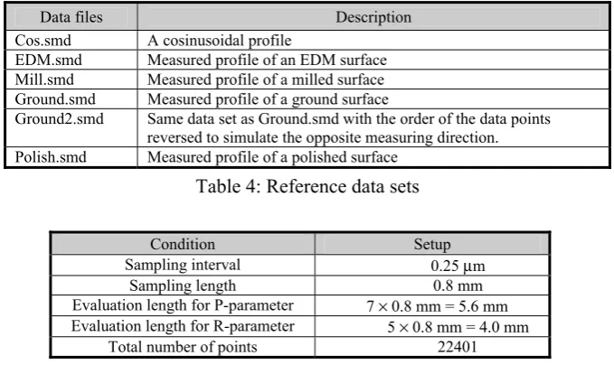
This comparison used six reference data sets as listed in Table 4. The cosine wave has a wavelength of 160 μm and amplitude of 2 μm. To minimise the effect of sampling conditions on evaluation, the same sampling interval, number of sampling lengths and number of points are consistent over the six profiles (see Table 5). Based on the information gained from a consultation exercise [16], four measured surface profiles, a milled, a polished, an EDM and a ground surface were used to address industrial requirements. Use of measured profiles as the reference data sets can assess the variation caused by different software packages. Using a reference data pair can demonstrate the robustness of parameter definitions in ISO standards.

Data files Description

Cos.smd A cosinusoidal profile

EDM.smd Measured profile of an EDM surface Mill.smd Measured profile of a milled surface Ground.smd Measured profile of a ground surface

Ground2.smd Same data set as Ground.smd with the order of the data points reversed to simulate the opposite measuring direction. Polish.smd Measured profile of a polished surface

Table 4: Reference data sets

Condition Setup

Sampling interval 0.25 _μm

Sampling length 0.8 mm

Evaluation length for P-parameter 7 × 0.8 mm = 5.6 mm Evaluation length for R-parameter 5 × 0.8 mm = 4.0 mm

Total number of points 22401

Table 5: Profile measurement condition

4.2 Reference

result

profiles using in the comparison, the reference result is the non-weighted mean of results obtained from the three F2 standards.

4.3 The performance metrics for Cos.smd

Sinusoidal artefacts have been widely used in the calibration of surface measuring instruments since they were first introduced by Sharmen in 1967 [38]. Sinusoids are insensitive to many measurement conditions. Some research comparison results are listed in Table 6. To reproduce these research results, the effect of software is assumed to be insignificant. The metric for Ra is set based on the reproducibility of these research results from the respect of software.

No Reference1 _{Metric for}

Ra2

1

H. Haitjema (1998) estimated the uncertainty of roughness parameters using styles instrument [4]. It was shown that the uncertainty of Ra and RSm for a sinusoidal artefact (nominal Ra: 2.9 µm and RSm: 100 µm) are 0.25 % and 0.03 % (at 95 % confidence).

0.04 %

2

NIST F2 standard is able to simulate the measurement error by adding the normal distributed random noise to each data point. The uncertainty of Ra and RSm for Cos.smd (nominal Ra: 636.62 nm and

RSm: 160 µm) is ± 2.68 nm and ± 6.97 µm (at 95 % confidence).

0.07 %

3

T. Vorburger et. al. (2007) undertook a comparison between optical and stylus methods [5]. For a sinusoidal specimen (nominal Ra: 500 nm and RSm: 50 µm), the Sa - Ra differences was 6 nm obtained from difference type of instruments.

0.1 %

4

T Thomas (1982) investigated the (in)homogeneity of some typical manufactured surfaces [3]. The variation of 1.8~3 % for Ra were found on RTH reference standards (Two-dimension sinusoidal surfaces, nominal Ra: 0.27 µm).

0.6 %

Note: 1_{. Based on the assumption that software used in this research work is qualified.} 2_{. The pass margin set as 1/3 of value of uncertainty and 1/10 of absolute difference.}

Table 6: The performance metrics for Cos.smd

4.4 The performance metrics for measured profiles

Table 7 lists the percentage coefficients of variation from place to place on a manufactured surface studied by Thomas [3]. ISO 4288 introduces the “The 16 %-rule” and “The max.-rule” for comparison of the measured values within tolerance limits. For the measured profiles used in this comparison, we provide six significant digits that include false precision and guard digits. For measured profiles, the software effect is considered as insignificant when the relative difference of results obtains from the test software and a reference result is less than 0.5 %. Therefore, we set the “pass margin” as 0.5 % in this comparison.

Milled Ground

Ra /% 17 ~ 65 7~80

Rq /% 15 ~ 61 9 ~ 56

Rsk* 0.35 ~ 0.75 0.22 ~ 0.73

(Except* which is an absolute value)

5 Specification

variation

In the following sections the square brackets refer to the associated software packages or ISO documents.

5.1 Pre-process

operator

[CC]

Deletes the last point of the data set when inputting a data file. [CB]

Adds an extra point when opening a data file. The method seems to (by analysing the output file):

• Add an extra point in the middle of the profile.

• Change the height value of the last point to be equal to the penultimate point.

• Adjust the value of the spacing to keep the sampling length consistent. Comments:

The behaviour of [CB] and [CC] suggests that they implement a conversion between a point-based length definition and an interval-point-based length definition (see Section 5.6.1).

5.2 Levelling

[PTB]

The least-squares method is a mandatory operator. [NPL]

The start point of a software measurement standard is the primary profile that does not contain form errors.

[Others]

The least-squares method is an optional operator. Comments:

Levelling is the operator to remove tilt from a profile. The least-squares method is widely used in industrial practice. However, conventional least-squares is not an appropriate method for a sine wave [39], and the least-squares normal method is more appropriate [40].

5.3 Evaluation length and sampling length

5.3.1 R-parameters

5.3.1.1 End effect of filtering

See Appendix C.2.

5.3.1.2 RSm

[ISO]

RSm is defined within a sampling length. [NPL][PTB]

Comments:

There is no mandatory method to reduce the end effects of the filtering operators9_{, thus different}

types of filters could cause different parts of a measured profile to be evaluated.

Defining the RSm parameter over the evaluation length will deliver a more stable result (see Section 5.5).

5.3.2 P-parameters

[ISO]

lp is equal to the length of the feature being measured. [PTB][CA]

lp(default): The remaining profile after removing one λc cut-off at each end of profile [NPL][NIST][PTB][CB][CC]

lp(default): All the measured points in a data file. Comments:

For interpretation of CA, it should be noticed that:

• Currently, there is no standardised method to reduce the end effect of a filtering operator.

• The value of a P-parameter will depend on the selection of the λc value.

Thus, to avoid ambiguity, this interpretation requires specifying the λc value when stating the P -parameters (it does not follow ISO 1302: 2000).

5.3.3 W-parameters

There is no common understanding of the meaning and use of waviness parameters [39]. ISO 4287 defines the sampling length of W-parameters based on the cut-off of the profile filter λf. Some industrial practice ignores this filter step and uses a sampling length λw equal to the cut-off wavelength λc.

5.4 Filtering

5.4.1 λs filtering

[CC]

The λs profile filtering is a mandatory part of the λc profile filtering (following ISO 3274 - Table 1).

[Others]

The λs profile filtering is an optional operator (ISO 4287).

5.5 Profile

element

5.5.1 Joint direction

[ISO]

A profile element is defined as a peak with a following valley (ISO 4287: 1997 - figure 3), or a valley with a following peak (ISO 4287:1997 - figure 10).

[NIST]

9 _{There is a standard under development, ISO/CD TS 16610-28, Geometrical product specifications}

A profile element is defined as a peak with a following valley. Comments:

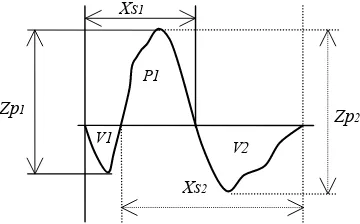
The ambiguity of ISO’s definition is shown in Figure 5. In this case, there are two valid profile elements with different height and width value. Profile element should be defined as a concept only. All the calculations should be defined based on features (a peak or a valley).

Figure 5: Ambiguity of the definition of profile element, the height and width of the profile element could be 1) Zp2and Xs2; 2) Zp1and Xs1; 3) (Zp2+Zp1)/2 and (Xs2+ Xs1)/2

5.5.2 Incomplete portion

[ISO]

The incomplete portion is the feature at the beginning or end of a sample length (e.g. the gray areas in Figure 6), and a handling method is provided as:

“The positive or negative portion of the assessed profile at the beginning or end of the sampling length should always be considered as a profile peak or as a profile valley. When determining a number of profile elements over several successive sampling lengths, the peaks and valleys of the assessed profile at the beginning or end of each sampling length are taken into account once only at the beginning of each sampling length.” (ISO 4287: 1997 Clause 3.2.7)

[PTB][NIST][NPL]

The NMIs do not follow the definition according to ISO due to its ambiguity. [NPL][PTB]

Assess the RSm and PSm parameters within the evaluation length and discard the incomplete portion at each end of the evaluation length.

Comments:

Figure 6 illustrates the imperfection of the ISO definition.

Sampling Length

Measuring Direction

RSm

/mm

l1 0.4

l1  0.4

l2  0.375

l2 0.325

Figure 6: Ambiguity of definition of the incomplete portion: results vary from 0.325 mm to 0.4 mm while the true value is the 0.4 mm in this case

Sampling Length l1

Xs1 Xs2

Xs3

Sampling Length l2 Xs4 Xs5

0 0.4 0.8

V1

Xs1

Xs2

Zp1 _Zp

2

P1

5.5.3 Insignificant features

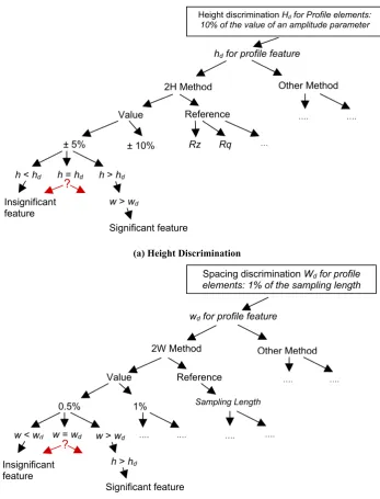
5.5.3.1 Identification of insignificant feature

[ISO]

Height discrimination (Hd) for profile elements: 10 % of the value of an amplitude parameter. Spacing discrimination (Wd) for profile elements: 1 % of the sampling length.

[NPL]

2H method (see Figure 7):

Height discrimination (hd) for profile feature: ± 5 % of Rz.

Spacing discrimination (wd) for profile feature: 0.5 % of sampling length.

Figure 7: NPL’s implementation of 2H method for height and spacing discrimination [PTB]

2H method:

Height discrimination (hd) for profile feature: ± 5 % of Rq on the Internet portal.

The desktop version of the software (Ref_soft_PTBIDL) allows the setting of the vertical and horizontal discrimination. In this comparison the height discrimination of ± 5 % of Rz was used.

[NIST] 2H method:

Height discrimination (hd) for profile feature: ± 5 % of Rz. Comments:

To identify the insignificant features, the concept of discrimination of a profile element is introduced into ISO standards. The definition of profile element is ambiguous (see section 5.5.1). All the software implementations, thus, identify the insignificant peaks/valleys directly. There is a significant specification variation for applying discrimination to peak and valley as illustrated in Figure 8.

10 % of Rz

1% of Sampling length Discrimination for a profile element (ISO 4287)

2H Method

5 % of Rz Discrimination for a profile feature (NPL)

(a) Height Discrimination

(b) Spacing Discrimination

Figure 8: Ambiguity of discrimination

5.5.3.2 Handling method for insignificant feature

After being identified, the insignificant features can be classified in to five types by their position, that of:

1) insignificant features at each end of the sampling length, 2) insignificant features at each end of the evaluation length,

3) incomplete insignificant features at each end of the sampling length, 4) incomplete insignificant features at each end of the evaluation length and 5) insignificant features in the middle of the sampling length.

According to its type, an insignificant feature can be discarded or merged into its neighbouring feature.

[ISO]

There is no specified method for handling an insignificant feature. [NPL]

Spacing discrimination Wd for profile elements: 1% of the sampling length

2W Method _{Other Method}

0.5% 1%

w < wd

…. ….

w = wd w > wd

Value Reference

Sampling Length

…. ….

Insignificant feature

Significant feature

?

h > hd

wd for profile feature

…. ….

2H Method Other Method

± 5% ± 10%

hdfor profile feature

h < hd

…. ….

h = hd h > hd

Significant feature

Value Reference

Rz Rq …

?

w > wd

Height discrimination Hd for Profile elements:

10% of the value of an amplitude parameter

1) RSm is calculated over the evaluation length to reduce the number of type 1 and type 3 features.

2) Discard type 2 and type 4 features.

3) For type 5 features, start with the smallest segments and combine with two adjacent segments.

[PTB]

See the description of the calculation of XSm and Xc parameters on the Internet portal. Comments:

Figure 9 illustrates five combination algorithms for removing the type 5 insignificant features. The method 1), 2), 3), and 4) were studied by Leach and Harris and showed the difference of the results of RSm obtained by different methods could up to 12 % [41]. Scott proposed method 5 and proved its stability by the representation theory of measurement [42].

Figure 9: Ambiguity of combination method (the black points represent the crossing points of a profile)

5.6 Discrete

interpretation

5.6.1 Length definition

The total profile is defined in the digital form as a discrete profile (ISO 3274), while most definitions of further operations within ISO 4287 and ISO 11562 still take the continuous form. There are two typical discrete algorithms used to calculate the distance between two points in the horizontal direction (see Table 8).

Point-based definition Interval-based definition

Where n is the number of points between its ends, and i

is the sampling interval. The length as l calculated

( 1) l= − ×n i,

The length l calculated as

l= ×n i,

In mathematics, in a particular geometry, a distance function satisfies the following conditions:

1) d(x,y)≥0, and d(x,y)=0 if and only if x y= . 2) d x y( , )=d y x( , )

3) d(x,z)≤d(x,y)+d(y,z)

It satisfies condition 1,

2 and 3. It satisfies condition 1 only.

Table 8: Length algorithm

Table 9 lists the influence of the length definition in this testing. If the last point is a significant point such as a crossing point or the highest/lowest point, the effect will be significant. PTB and NIST use the interval-based definition in sampling length and evaluation length while NPL use a point-based definition. The two definitions are used in various ways in many software implementations.

(1)

(2) (5)

(3)

Data file ：Cos.smd Evaluation length: 5.6 mm sampling interval: 0.25 µm Lc: 0.8 mm

Ls: 2.5 um

Point-based definition Interval-based definition

The number of data points:

within a data profile 22401 22400

within a evaluation length 16001 16000

within a sampling length 3201 3200

The number of data points used to implement Gaussian weight convolution.

Ls filtering

Lc filtering 3201 11 3200 10

Table 9: The effect of the different length definition

Mean line crossing-points

[NPL]

Use a natural cubic spline to interpolate through the discrete data values. Comments:

The mean line is a base to which feature parameters are referred. Unfortunately, most of the mean line crossing-points are excluded in the measured data point set, and the position of a mean line crossing-point is generally estimated from its neighbouring points. Thus, there are many different algorithms to estimate a crossing-point and the method uncertainty is introduced to the final results. In addition, there is error when calculation based on the measuring data point set without those mean line crossing-points [43]. Brennan recommended the need to include implied mean line crossing points simply by interpolating the data where these occur and provide each profile peak or valley element with calculated boundary values.

5.7 Two

examples:

Ra

and

RSm

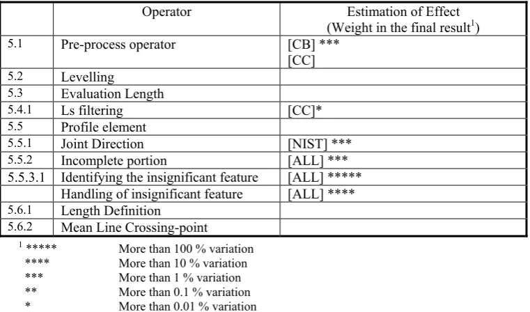
Table 10 and Table 11 estimate the effect of specification variation in the final result of test software.

Operator Estimation of Effect

(Weight in the final result1₎

5.1 Pre-process operator [CB] ***

[CC]

5.2 Levelling [PTB] *

5.3.1.1 End effect of Lc filtering [CC] *

5.4.1 Ls filtering [CC] *

5.6.1 Length Definition

5.6.2 Mean Line Crossing-point

1 _{***** More than 100 % variation}

**** More than 10 % variation *** More than 1 % variation ** More than 0.1 % variation * More than 0.01 % variation

Operator Estimation of Effect (Weight in the final result1₎

5.1 _{Pre-process operator [CB] ***}

[CC]

5.2 Levelling

5.3 Evaluation Length

5.4.1 Ls filtering [CC]*

5.5 Profile element

5.5.1 Joint Direction [NIST] ***

5.5.2 Incomplete portion [ALL] *** 5.5.3.1 Identifying the insignificant feature [ALL] *****

Handling of insignificant feature [ALL] ****

5.6.1 Length Definition

5.6.2 Mean Line Crossing-point

1 _{***** More than 100 % variation}

**** More than 10 % variation *** More than 1 % variation ** More than 0.1 % variation * More than 0.01 % variation

Table 11: The estimation of effect of specification variation for RSm

6 Evaluation and discussion

6.1 Evaluation of Cos.smd

Table 18 and Table 19 in Appendix B present results for Cos.smd obtained from the test software, together with the mean and standard deviation of the results.

6.1.1 Effect of levelling operator

For PTB’s type F2 standard and CB, the effect of the levelling operator is analysed in Appendix C.2. Due to the different length definition, the last point of Cos.smd is not taken into account by PTB’s type F2 standard and CB. Thus Pp is 0.04 nm less than the expected value while Pv is 0.04 nm greater.

6.1.2 Effect of filtering

Cos Cos Cos Cos Cos Cos Cos Cos Cos Cos Cos

|Pa-Ra| |Pq-Rq| |Psk-Rsk| |Pku-Rku| |Pp-Rp| |Pv-Rv| |Pz-Rz| |Pt-Rt| |Pc-Rc| |PSm-RSm| |Pdq-Rdq|

/nm /nm /nm /nm /nm /nm /nm /μm

NIST 1.0E-02 1.0E-02 1.3E-04 2.0E-05 0.0E+00 0.0E+00 0.0E+00 0.0E+00 0.0E+00 0.0E+00 2.0E-05

NPL 9.1E-06 1.0E-05 2.2E-09 1.0E-09 1.3E-03 1.5E-05 1.3E-03 6.5E-03 2.9E-05 0.0E+00 *

PTB 2.0E-02 3.0E-02 1.8E-04 0.0E+00 4.0E-02 4.0E-02 0.0E+00 0.0E+00 0.0E+00 0.0E+00 4.9E-05

CA 0.0E+00 1.0E+00 0.0E+00 0.0E+00 1.0E+00 1.0E+00 1.0E+00 1.0E+00 * * 1.9E-05

CB 1.8E+01 1.9E+01 8.8E-04 1.4E-04 2.7E+01 2.7E+01 5.5E+01 5.5E+01 8.5E+01 2.9E+00 8.0E-04

CC 3.0E-01 4.0E-01 1.0E-04 0.0E+00 6.0E-01 5.0E-01 1.1E+00 9.0E-01 1.1E+00 4.6E-01 1.7E-05

1) There are some missing points due to zero values cannot be plotted in this log chart. 2) Some results may be overstated or understated due to rounding effect.

Figure 10:Effect of filtering

6.1.3 RSm/PSm

The value of PSm/RSm should be 160 µm, which is the “true” value for this cosine wave. If we strictly adhere to ISO 4287: 1997, to evaluate within every sampling length and discard incomplete portions at the end of sampling length,

RSm = 152 µm and PSm = 158.857 µm.

If, following ASME B46.1-2002 [22], we evaluate within the evaluation length and discard incomplete portions at the end of evaluation length,

RSm = 158.4 µm.

If we use the interval-based length definition to define the sampling length, and the point-based length definition to calculate the width of a profile element within each sampling length, and discard the incomplete portions at each ends,

RSm = 159.95 µm.

If we use the interval-based length definition to define the evaluation length, and the point-based length definition to calculate the width of a profile element within the evaluation length, and discard the incomplete portions at each ends,

RSm = 159.99 µm.

Table 12 presents the PSm/RSm results for Cos.smd. It shows that NIST, NPL, PTB and CA have fixed the distortion introduced by ISO 4287. Commercial package CC adheres to ASME B46.1-2002. CB delivers significantly different results. PTB’s and NPL’s type F2 standards perform well in this test. PTB’s type F2 standard delivers a small error due to a different length definition.

PSm /µm RSm /µm

NIST 160.00 160.00

NPL 160.00 160.00

PTB 159.99 159.99

CA - 160.00

CB 158.89 156.01

CC 158.86 158.40

Table 12: Influence of incomplete portion for RSm and PSm

6.1.4 Computational error

results where only last digits are inaccurate. NPL’s type F2 standard delivers seven to ten accurate significant digits in this case, even higher than the precision of measuring data. For commercial packages, the level of precision reduces significantly with the range of LRE values falling between 1.6 to 4.6. Some of the results provide two to four false significant digits. Commercial package CB provides less than two accurate significant digits.

(The red line indicates the significant digits of the measuring data within data file.)

Figure 11: The number of correct significant digits

6.1.5 Software effect

Table 13 presents the software effect by comparing variation due to different software and data errors. The mean standard deviations of the results for Cos.smd obtained from different software have been used. These are compared to the measurement uncertainty due to data errors calculated by the NIST software. The software variation among the three software measurement standards is small compared with the data uncertainty. The exception to this is the RSm

parameter and Rc parameter due to their ambiguous definitions within standards. When commercial packages are compared , the software variations are significant.

Parameter Ra Rq Rku Rp Rv Rz Rt RSm Rdq1

Uncertainty calculated by NIST software2

Mean value R x 636.59 706.93 1.5009 1012.62 1012.94 2024.96 2035.69 160.33 0.0288

Uc(Rx) 1.34 1.09 0.003 1.72 1.74 2.53 4.16 3.49 0.00063

Deviation by 3 software measurement standards

∆Rx 0.02 1.3E-02 4.6E-08 6.2E-04 6.9E-06 6.2E-04 3.1E-03 4.7E-03 5.0E-06

∆Rx/uc(Rx)/% 1.53 1.23 0.00 0.04 0.00 0.02 0.07 0.14 0.79

Deviation by all software (3 software measurement standards and 3 industrial packages)

∆Rx 6.56 7.20 6.0E-05 10.21 10.21 20.34 20.34 1.49 0.00

∆Rx/uc(Rx)/% 489.33 660.39 1.99 593.82 586.89 803.90 489.06 42.61 49.34

Deviation by all software without industrial package CB

∆Rx 0.22 0.43 3.9E-08 0.52 0.49 0.66 0.60 0.64 0.00

∆Rx/uc(Rx)/% 16.61 39.38 1.29E-03 29.96 28.16 26.27 14.45 18.31 2.92

Note: 1 _{Parameter Rdq without NPL}

2 _{See Table 6.}

Table 13: Software effect vs. data effect

6.1.6 Fitness for purpose

NIST NPL PTB CA CB CC

Task 1,2,3,4 1,2,3,4 1,2,3,4 2,3,4 None 2,3,4

Table 14: The performance of software implementations for Ra of Cos.smd (assessed by the effect of the reproducibility of measurement tasks listed in Table 610₎

6.2 Evaluation of measured profiles

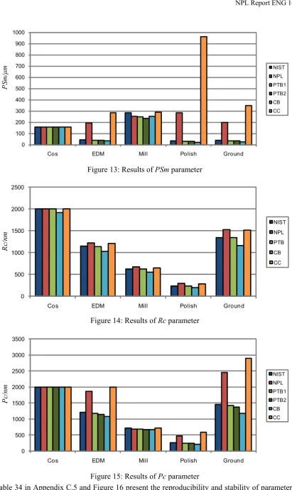
Table 20 to 24 in Appendix B present results for measured profiles obtained from test software, together with the mean and standard deviation of the results. Figure 17 to 38 in Appendix C show the relative differences between test results and reference results. Table 15 and 16 present the percentage of coefficients of variation among the three type F2 standards and three commercial packages. For the three type F2 standards, most of the relative differences are less than 0.5 %. NPL’s type F2 standard delivers slightly greater values of Rp, Rv, Rz, Rt, Pp, Pv, Pz

and Pt due to its interpolating method, and only one result is greater than 0.5 % (Rp for Polish.smd). For PSm, RSm, Pc and Rc, variations are significant as the result of ambiguous definition (see Figure 12-15). Together with the three commercial packages, most of relative differences for R-parameters are more than 0.5 %.

Ra Rq Rsk Rku Rp Rv Rz Rt Rc RSm Rdq

Cos.smd 0.00 0.00 - 0.00 0.00 0.00 0.00 0.00 0.00 0.00 0.02 EDM.smd 0.00 0.14 0.19 0.06 0.05 0.06 0.06 0.05 3.18 6.95 0.02 Mill.smd 0.00 0.15 0.12 0.01 0.14 0.18 0.16 0.13 3.78 7.10 0.07 Polish.smd 0.01 0.13 0.03 0.02 0.38 0.13 0.17 0.15 10.76 24.98 0.04 Ground.smd 0.00 0.25 0.13 0.00 0.05 0.03 0.04 0.02 6.39 16.66 0.01

Table 15: Percentage of coefficients of variation among three type F2 standards

Ra Rq Rsk Rku Rp Rv Rz Rt Rc RSm Rdq

Cos.smd 1.03 1.02 - 0.00 1.03 1.03 1.02 1.02 1.72 0.93 1.13 EDM.smd 1.03 1.36 30.17 0.89 7.10 5.65 2.71 0.60 6.10 9.08 2.31 Mill.smd 2.60 2.32 8.19 2.85 5.59 12.28 1.69 1.19 6.25 45.41 17.17 Polish.smd 1.03 1.21 1.29 1.98 7.30 7.95 3.11 1.24 13.66 33.77 9.12 Ground.smd 0.80 0.84 15.90 2.12 13.90 7.03 1.24 0.62 9.91 22.30 4.37

Table 16: Percentage of coefficients of variation among three type F2 standards and commercial packages

0 50 100 150 200 250 300

Cos EDM Mill Polish Ground

RS

m

/

μ

m NIST

NPL PTB CA CB CC

Figure 12:Results of RSm parameter

0 100 200 300 400 500 600 700 800 900 1000

Cos EDM Mill Polish Ground

PS

m

/

μ

m NIST

NPL PTB1 PTB2 CB CC

Figure 13: Results of PSm parameter

0 500 1000 1500 2000 2500

Cos EDM Mill Polish Ground

Rc

/n

m

NIST NPL

PTB CB CC

Figure 14:Results of Rc parameter

0 500 1000 1500 2000 2500 3000 3500

Cos EDM Mill Polish Ground

Pc

/n

m

NIST NPL PTB1 PTB2 CB CC

Figure 15:Results of Pc parameter

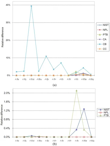
0.05 %, while the difference of Rc and RSm fall with the range of 2.1 % and 0.76 %. For commercial package CA and CC, the relative difference of RSm is 1 % and 0.64 %. Commercial package CB delivers significant errors for all parameters, the relative difference is up to 40 %.

(a)

(b)

Figure 16: The effect of direction

7 Conclusions

In general the results for R-parameters obtained from the three type F2 standards are in good agreement. The exceptions are the RSm and Rc parameters. The reason for this disagreement is the ambiguous and unstable definitions given within ISO standards. The three software measurement standards performed better than the three commercial packages by giving high precision results and their specifications adhere closely to ISO standards.

software packages is even greater than the variation caused by the surface inhomogeneity, variation of measurement environment and different data collection methods. Therefore, it is not safe to ignore the calibration of software embedded within a surface instrument. Some particular conclusions are as follows:

• The current specifications of parameters Ra, Rq, Rsk, Rp, Rt and Rz are clearly defined and stable. The three type F2 software standards are qualified to provide accredited results for those parameters for commercial packages.

• The specifications of parameters RSm and Rc are ambiguous and unstable. The variation of RSm is significant. The revised specification of RSm proposed by Scott [42] is mathematically stable in this test.

• The specifications of P-parameters are unambiguous in standard documents. However, there are different understandings of the meaning of P-parameters, which leads to different interpretations.

• The effect of rounding error is insignificant in the test. The major contributor to the variation is the specification variation.

In addition, there are significant variations on the results of W-parameter as well11.

8 Reference:

1. Jiang, X., et al., Paradigm shifts in surface metrology. Part I. Historical philosophy.

Proceedings of the Royal Society A: Mathematical, Physical and Engineering Sciences, 2007. 463(2085): p. 2049-2070.

2. Jiang, X., et al., Paradigm shifts in surface metrology. Part II. The current shift.

Proceedings of the Royal Society A: Mathematical, Physical and Engineering Sciences, 2007. 463(2085): p. 2071-2099.

3. Thomas, T.R. and G. Charlton, Variation of roughness parameters on some typical manufactured surfaces. Precision Engineering, 1981. 3(2): p. 91-96.

4. Haitjema, H., Uncertainty analysis of roughness standard calibration using stylus instruments. Precision Engineering, 1998. 22(2): p. 110-119.

5. Vorburger, T., et al., Comparison of optical and stylus methods for measurement of surface texture. International journal of advanced manufacturing technology, 2007. 33: p. 110-118.

6. Song, J.F. and T.V. Vorburger, Standard reference specimens in quality control of engineering surfaces. J. Res. Natl. Inst. Stand. Technol., 1991. 96: p. 271-289.

7. Scott, P.J., Developments in surface texture measurement. Surface Topography, 1988. 1: p. 153-163.

8. Stout, K.J., et al., The Development of Methods for the Characterization of Roughness in Three Dimensions. 1993, Luxembourg: Publication No. EUR 15178 EN of the Commission of the European Communities.

9. Bui, S.H., et al. Surface metrology software variability in two-dimensional

measurement. in Pro. ASPE 2003. 2003.

10. Bui, S.H., et al., Internet-based surface metrology algorithm testing system. Wear, 2004. 257(12): p. 1213-1218.

11. Euromet600 - Final Report. Euromet Project 600 – comparison of surface roughness standards. 2004 Available from:

www.bipm.org/utils/common/pdf/final_reports/L/S11/EUROMET.L-S11.pdf.

11 _{We do not present the results of W-parameters in this report because they are seldom used}

12. ISO 5436-1:2000, Geometrical Product Specifications (GPS) -- Surface texture: Profile method; Measurement standards -- Part 1: Material measures: International Organization for Standardization.

13. ISO 5436-2:2001, Geometrical Product Specifications (GPS) -- Surface texture: Profile method; Measurement standards -- Part 2: Software measurement standards: International Organization for Standardization.

14. Jung, L., et al. Reference software for roughness analysis-features and results. in The XI international colloquium on surfaces. 2004. Shaker Verlag.

15. Bui, S.H. and T.V. Vorburger, Surface metrology algorithm testing system. Precision Engineering, 2007. 31(3): p. 218-225.

16. Blunt, L., et al., The development of user-friendly software measurement standards for surface topography software assessment. Wear, 2008. 264(5-6): p. 389-393.

17. ISO/IEC TR 9126-2:2003, Software engineering – Production Quality – Part 2: External metrics: International Organization for Standardization.

18. IEC BIPM ISO IFCC I IUPAC, Guide to the expression of uncertainty in measurement. 1995, Geneva.

19. ISO TC213. ISO 2004 Business Plan of ISO/TC213. 2004 [cited; Available from: http://isotc213.ds.dk.

20. 17450-2:2002, I.T., Geometrical product specifications (GPS) -- General concepts -- Part 2: Basic tenets, specifications, operators and uncertainties.

21. ISO/IEC Guide 99:2007, International vocabulary of metrology -- Basic and general concepts and associated terms (VIM): International Organization for Standardization. 22. ASME B46.1-2002, Surface texture (surface roughness, waviness, and lay), New York:

Am Soc Mech. Eng.

23. NPL. Specification of parameters. Softgauges for Surface Topography [cited; Available from: http://161.112.232.32/softgauges/pdf/Specification.pdf.

24. Mari, L. On the measurand definition. in XVIII IMEKO world congress. 2006. Rio de Janeiro, Brazil

25. Phillips, S.D., et al., A Careful Consideration of the Calibration Concept. J. Res. Natl. Inst. Stand. Technol., 2001. 106: p. 371-379.

26. Ehrlich, C., R. Dybkaer, and W. Wöger, Evolution of philosophy and description of measurement (preliminary rationale for VIM3). Accreditation and Quality Assurance: Journal for Quality, Comparability and Reliability in Chemical Measurement, 2007. 12(3): p. 201-218.

27. Baratto, A.C., Measurand: a cornerstone concept in metrology. Metrologia, 2008. 45(3): p. 299-307.

28. Pavese, F., The definition of the measurand in key comparisons: lessons learnt with thermal standards. Metrologia, 2007. 44(5): p. 327-339.

29. McCullough, B.D., Assessing the Reliability of Statistical Software: Part I. The American Statistician, 1998. 52(4): p. 358-366.

30. NIST. STRD- Statistical Reference DatasetsAvailable from: http://www.nist.gov/itl/div898/strd.

31. McCullough, B.D., Special section on Microsoft Excel 2007. Computational Statistics & Data Analysis, 2008. 52(10): p. 4568-4569.

32. McCullough, B.D. and D.A. Heiser, On the accuracy of statistical procedures in Microsoft Excel 2007. Computational Statistics & Data Analysis, 2008. 52(10): p. 4570-4578.

33. McCullough, B.D. and B. Wilson, On the accuracy of statistical procedures in Microsoft Excel 97. Computational Statistics & Data Analysis, 1999. 31(1): p. 27-37. 34. McCullough, B.D. and B. Wilson, On the accuracy of statistical procedures in

Microsoft Excel 2003. Computational Statistics & Data Analysis, 2005. 49(4): p. 1244-1252.

35. Cox, M.G. and P.M. Harris, Design and use of reference data sets for testing scientific software. Analytica Chinmica Acta, 1999. 380(2-3): p. 339-351.

37. Lines, K.J., F.O. Onakunle, and I.M. Smith, Testing functions for calculation the discrete Fourier transform and its inverse, in NPL Report. 2007, National Physical Laboratory: London.

38. Sharman, H.B., Calibration of surface texture measuring instruments, in Proceedings of the Institution of Mechanical Engineers. 1967, Journal of engineering manufacture. p. 319.

39. Whitehouse, D.J., Surfaces and Their Measurement. 2002: Taylor & Francis.

40. Murthy, T., G. Reddy, and V. Radhakrishnan, Different functions and computations for surface topography. Wear, 1982. 83: p. 203-214.

41. Leach, R.K. and P.M. Harris, Ambiguities in the definition of spacing parameters for surface-texture characterization. Measurement Science and Technology, 2002(12): p. 1924.

42. Scott, P.J., The case of surface texture parameter RSm. Measurement Science and Technology, 2006(3): p. 559.

9 Appendix A: Measurement conditions

Form Removed

The form removal operation is set as standard in PTB’s F2 standard, is an option in NIST’s F2 standard, and is not used in NPL’s F2 standard. Therefore, in this test, all measured reference data sets were levelled by the least-squares straight line method on NIST F2 standards before input into all F2 software standards and commercial packages.

Filtering

At the filtration stage, we used only a Gaussian filter with long-wavelength cut-off λc of 0.8 mm calculated by the convolution method.

Sampling Length and Evaluation Length

To minimise the distortion due to the convolution filter, one cut-off at each end of the roughness profile is normally removed. All data sets include 7 cut-offs and the evaluation of the R-parameters is based on the middle five cut-offs. P-parameters are calculated based on all data points in files and, therefore the evaluation length of P-parameters is equal to 5.6 mm in these profiles.

Parameters

The parameters to be compared here are defined by ISO 4287: 1996. The waviness profile is not well defined in current ISO standards due to there is no common understanding of the meaning and use of waviness parameters. Thus, the comparison of W-parameters calculation is not very meaningful and is not discussed in the report.

File format

It should be noted that some test used different data file format due to some software packages do not support SMD data format. In some case, data type is converted and precision is reduced.

The variation of measuring condition

Variation of measuring conditions is listed in Table 17.

PTB NIST NPL CA CB CC

Levelling LSQ LSQ

Profile filtering λs