Multi objective Optimization of Transmission Line Annual Maintenance Scheduling Based on Flower Pollination Algorithm

2017 International Conference on Computer Science and Application Engineering (CSAE 2017) ISBN: 978-1-60595-505-6

Multi-objective Optimization of Transmission Line Annual

Maintenance Scheduling Based on Flower Pollination Algorithm

Song Xianyong and Shen Quanyu*

Power Dispatching Control Center, Yueyang Power Supply Company of State Grid, 414001 Yueyang, China

ABSTRACT

The optimization of the annual maintenance scheduling is a multidimensional and nonlinear integer optimization problem. In this paper, the annual maintenance scheduling model is established with the minimum cost of maintenance and the expected minimum power supply, and the pollination algorithm based on e constraint is proposed. By obtaining the Pareto optimal solutions and comparing the economic and reliability objectives of the optimization problem of the maintenance scheduling, the proposed algorithm can effectively improve the solution precision of the multi - objective optimization problem and the distribution of the optimal solution. Based on the annual inspection scheduling of 12 transmission lines in a region, this paper compares the proposed algorithm with the Differential Evolution Flower Pollination Algorithm with Time Variant Factor (TVDFPA) and the Simulated Annealing Pollination Algorithm (SFPA). Based on the result, ε-constrained algorithm is superior to the other two in performance and calculation time.

INTRODUCTION

State maintenance is the use of modern technology to monitor the equipment, the current conditions for the equipment to determine the best maintenance time maintenance methods[1,2]. In this paper, with the economic, reliability, security as the goal, the use of relevant mathematical methods for constraint processing and solution, the main purpose is to develop a more reasonable and targeted maintenance program. Compared with the traditional transmission line regular maintenance method, this method saves a lot of maintenance costs, and can increase the reliability of transmission lines, more in line with the current power enterprise operation and management requirements.

the Benders decomposition method, the sensitivity analysis method and the reliability analysis method in the transmission line maintenance and the comparison between the advantages and disadvantages of the algorithm. The optimization algorithm should be based on the calculation speed and convergence as the main improvement direction.

In this paper, we use the ε-constrained processing method and the pollination algorithm to improve the original pollination algorithm and establish a multi-objective optimization model for the maintenance model of the transmission line. The multi-objective optimization model of the line maintenance model is established. TVDFPA and SFPA are compared with the proposed method. The results show that the improved algorithm can improve the efficiency and reduce the time of calculation.

MULTI-OBJECTIVE OPTIMIZATION METHOD Pollination Algorithm

Pollination algorithm is used in power system to solve the optimal solution by diminishing certain performance. In the literature [9,10], pollination algorithm are used for optimal allocations and sizing of capacitors in various distribution systems. In the literature [11], researchers use it to find out the optimal parameters of a static VAR compensator. In the literature [12], combined economic emission dispatch problem in power systems is suggested to be solved by the pollination algorithm.

The principle of pollination algorithm [13] is to imitate the pollination process of flowers. Combined with Levy flight [14], it is able to achieve local search and global search, with fewer parameters, fast calculation characteristics.

The following are four rules for the pollination.

1) Biological cross flower pollination as a global pollination, pollination mode is considered Levi flight.

2) Local pollination uses non - biological pollination and self - pollination.

3) Pollinators, such as insects, will develop the habit of patronizing a particular flower, and its breeding probability is proportional to the similarity of a two flowers.

4) Local pollination and global pollination are controlled by the transfer probability, which is slightly biased towards local pollination.

According to rule 1 and rule 3, the global pollination of the position change is updated as follows:

1

( )( )

t t t

i i i

x  x

 

L gx ₍₁₎

In this paper, L(λ) is used to simulate the movement of insects. The paper used Levi flight L(λ)> 0 Levi distribution:

L~ ( )sin( / 2) 1₁ (s 0)

s 

  

 

 _

(2)

The distribution of Γ(λ) is effective for larger steps (s>0). Using the Mantelia algorithm [14] to calculate the step size s:

2

1/ , ~ 0, ~ (0,1)

U

s U V N

V 



 （ ）， ₍₃₎

1 2

( 1)/ 2 (1 ) sin( / 2) [(1 )/2] 2





 



  

   

_  _

  

 ₍₄₎

For a given parameter λ, σ2 is a constant.

According to rule 2 and rule 3, the local pollination position changes the formula:

1

+ (

)

t t t t i i j k

x





x



x



x

(5)

Constraint Processing Method

ε-constrainted processing was first proposed by Takahama in 2005 [15], and its basic principle is similar to the feasible solution constrained constraint, except that it relaxes the constraint violation through the function at the early stage of the search. The method will produce more infeasible solutions in the early stages of optimization, and will be updated until the number of iterations has been reached. After the number of iterations reached Tc, the constraint processing is the same as the feasible solution constrained constraint processing. The ε function is updated according to the following formula:

(0)(1 ) ,0

( )

0, cp

c c

c

k

k T T

k

k T 



 _{  }

  

 _

 ₍₆₎

(0)

v x

(

_

)





₍₇₎

the reference range of cp is [2,10].

Multi - Objective Optimization Algorithm Performance Index

Judging the quality of multi-objective optimization problems, there are usually two indicators:

1) The degree of convergence of the solution set to the true Pareto solution set. 2) the diversity of solutions.

In order to quantify the multi-objective optimization algorithm, this paper uses the performance index function R(IR2) :

2

( , ) ( , )

R

u A u R

I   

 

 







(8)

A MULTI - OBJECTIVE OPTIMIZATION MODEL FOR TRANSMISSION LINE STATE MAINTENANCE

Multi - Objective Optimization Model

1 2 3

' ' '

min ( ) [ ( ), ( ), ( )]

( ) 0,( 1, 2,..., )

( ) 0,( 1, 2,..., )

NT NT NT NT

j kt r

p kt r

i kt i

y f f f f

g x j k

h x p l

l x u

 

  

     

X X X X

(9)

In the formula, xkt’=1 means overhaul, xkt’=0 means not overhauled. Pareto Optimal solution definition can be listed as：

If and only when 1 2

1 2

( ) ( ), 1, 2,...,

( ) ( ), 1, 2,...,

i i

i i

f X f X i m

f X f X i m

  

   (10)

A solution that is not dominated by any solution is the Pareto optimal solution, which is usually a solution set.

Objective Function

Transmission line condition maintenance plan arrangements, it is necessary to consider its economic indicators, while meeting the requirements of the system reliability. Therefore, the general optimization of transmission line maintenance scheduling has two objectives, namely, economic objectives and reliability objectives.

(1) Economic objective function based on life cycle theory.

1

1 1

( ) /

T N

kt kt kt kt t k

f x C x 

  



 (11) kt kt k k L T U   (12) In the formula, Tk includes installation costs, design costs, material costs,

transportation costs.

(2) Reliability objective function based on ETS evaluation of expected power supply.

1 3

1 1

( ) ( kt(1 ) kt)

t

N T

x x

kt x k k t

t x S k

f x L P P  T

  



  



(13) Restrictions

(1) Restrictions on the maintenance of the constraint conditions associated with the transmission line overhaul strategy:

1

0 or

kt k k

kt k k

x e t l

x t e t l

    

 _{    }

 ₍₁₄₎ While the maintenance of the constraints:

1 2 ... n

k t k t k t

x x  x n

or xk t1 xk t2  ... xk tn 0 ₍₁₅₎

Mutual restraint:

0 x it xjt 1 (16)

Sequential maintenance of the constraint

j i i

t  t T (17)

1 0

kt

x  _or x_kt2 0 ₍₁₈₎ Maintenance of resources constraints:

Human resource constraints are:

1

T

kt kt t t

h x H







(19) The resource constraints are:

1

T

kt kt t t

r x R







(20) Reasonable allocation of constraints for each period of maintenance:

1

N

k kt t k

m x M







(21) Special weather constraints:

1

e kt

x  (22)

(2) Constraints relating to the stability of transmission lines Transmission path constraint:

_{kt r}

k r

x b







(23) In the formula, the total number r of different transmission path lines formed by the collection is different.

i i i i NG i NC i NC

PG C PD

  

 







(24)

( ) o

A PGPCPD T ₍₂₅₎

Excessive level of risk:

(Rk Rst)

Count _   K

(26) In the formula, the upper limit δ is based on the critical degree of the line in the network. Once the risk assessment result of the line exceeds the upper limit, it needs to be repaired immediately. K represents the total number of lines.

EXAMPLE ANALYSIS

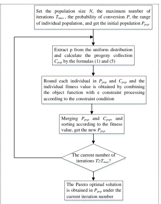
Round each individual in Ppop and Cpop and the

individual fitness value is obtained by combining the object function with e constraint processing according to the constraint condition

Merging Ppop and Cpop, and

sorting according to the fitness value, get the new Ppop

The current number of iterations TTmax?

Set the population size N, the maximum number of iterations Tmax , the probability of conversion P, the range

of individual population, and get the initial population Ppop

Extract p from the uniform distribution and calculate the progeny collection

Cpop by the formulas (1) and (5)

The Pareto optimal solution is obtained in Ppop under the

[image:6.612.134.464.46.465.2]

current iteration number

Figure 1. Flow chart of multi-objective optimization process.

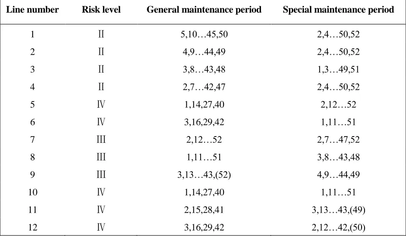
According to the transmission line state maintenance method to develop the 12 lines of the maintenance scheduling. To develop the transmission line annual maintenance scheduling, for example, the time t unit for the week, a total of 52 maintenance period, that is, T is 52. The initial arrangement of the state maintenance scheduling is shown in TABLE II.

[image:7.612.87.507.81.330.2]

TABLE I. PARAMETERS OF TRANSMISSION LINES BASED ON CONDITION EVALUATION AND RISK ASSESSMENT.

Line

number Voltage level Status level Risk level

Overhaul length (km)

Total number of

towers

1 500kV attention Ⅱ 32.443 86

2 500kV attention Ⅱ 28.887 77

3 500kV attention Ⅱ 15.115 33

4 500kV attention Ⅱ 15.115 33

5 220kV attention Ⅳ 45.55 117

6 220kV normal Ⅳ 4.73 16

7 220kV normal Ⅲ 4.88 17

8 220kV abnormal Ⅲ 43.62 127

9 220kV abnormal Ⅲ 29.82 84

10 220kV normal Ⅳ 12.265 43

11 220kV normal Ⅳ 5.26 22

12 220kV attention Ⅳ 25.204 75

TABLE II. ORIGINAL SCHEDULING OF TRANSMISSION LINE CONDITION-BASED MAINTENANCE.

Line number Risk level General maintenance period Special maintenance period

1 Ⅱ 5,10…45,50 2,4…50,52

2 Ⅱ 4,9…44,49 2,4…50,52

3 Ⅱ 3,8…43,48 1,3…49,51

4 Ⅱ 2,7…42,47 2,4…50,52

5 Ⅳ 1,14,27,40 2,12…52

6 Ⅳ 3,16,29,42 1,11…51

7 Ⅲ 2,12…52 2,7…47,52

8 Ⅲ 1,11…51 3,8…43,48

9 Ⅲ 3,13…43,(52) 4,9…44,49

10 Ⅳ 1,14,27,40 1,11…51

11 Ⅳ 2,15,28,41 3,13…43,(49)

12 Ⅳ 3,16,29,42 2,12…42,(50)

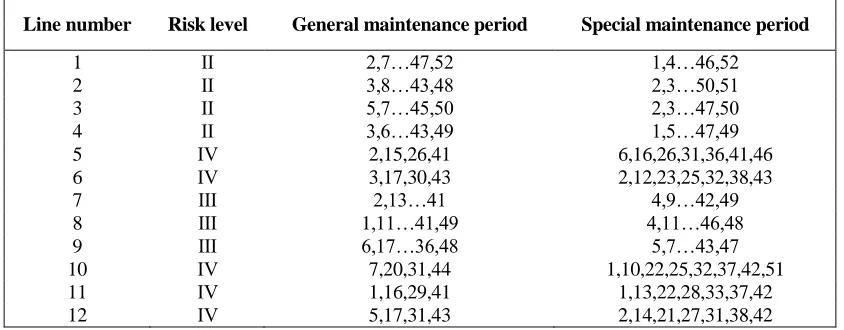
From the Pareto solution set of the daily maintenance optimization results, the highest ranking of the three plans, and compared with the initial maintenance scheduling, the economic and reliability indicators in TABLE IV.

[image:7.612.89.505.374.616.2]

[image:8.612.87.509.120.285.2]

lines. The resulting Pareto optimal solution matrix achieves better economic and reliability over the initial state maintenance scheduling matrix.

TABLE III. OPTIMIZATION OF TRANSMISSION LINE CONDITION-BASED MAINTENANCE SCHEDULING.

Line number Risk level General maintenance period Special maintenance period

1 Ⅱ 2,7…47,52 1,4…46,52

2 Ⅱ 3,8…43,48 2,3…50,51

3 Ⅱ 5,7…45,50 2,3…47,50

4 Ⅱ 3,6…43,49 1,5…47,49

5 Ⅳ 2,15,26,41 6,16,26,31,36,41,46

6 Ⅳ 3,17,30,43 2,12,23,25,32,38,43

7 Ⅲ 2,13…41 4,9…42,49

8 Ⅲ 1,11…41,49 4,11…46,48

9 Ⅲ 6,17…36,48 5,7…43,47

10 Ⅳ 7,20,31,44 1,10,22,25,32,37,42,51

11 Ⅳ 1,16,29,41 1,13,22,28,33,37,42

12 Ⅳ 5,17,31,43 2,14,21,27,31,38,42

TABLE IV. THE COMPARISON OF PARETO SOLUTION AND ORIGINAL SOLUTION OF DAILY MAINTENANCE.

Pareto optimal solution matrix economic reliability (EENS/MWh)

Xm=1,best 136 633.7 683.261 2

Xm=2,best 136 092.5 685.291 0

Xm=3,best 135 806.3 689.096 3

X 140 446.8 693.151 1

TVDFPA uses improved step factor, and the difference evolution strategy is added in the iterative process [16]. SFPA uses the simulated annealing (SA) to improve the global search capability of traditional flower pollination algorithm (FPA) [17]. These two methods and the method proposed in this paper are used to calculate the examples. The population size is 200 and the number of iterations is 1000. The performance index function R(IR2) and the calculation time results are shown in TABLE V and TABLE VI.

TABLE V. COMPARISON OF R INDICATOR.

R(IR2) ε-FPA TVDFPA SFPA

Best value 0.0136 0.0248 0.0236

Worst value 0.0246 0.1212 0.1236

Average value 0.0153 0.0811 0.0932

TABLE VI. COMPARISON OF COMPUTATION TIME.

time(s) ε-FPA TVDFPA SFPA

Best value 191.532 197.787 199.243

Worst value 193.246 199.643 203.458

Average value 192.343 198.854 200.009

CONCLUSIONS

In this paper, the constraint processing method and the pollination algorithm are combined to improve the original pollination algorithm., Simulated Annealing Pollination Algorithm (SFPA), and the Method of Differential Propagation Pollination Algorithm (TVDFPA) are compared in the two aspects of performance and calculation time. Methods were compared and the following conclusions were obtained:

(a) The improved pollination method proposed in this paper improves the local convergence problem, uses less algorithm parameters, and can effectively deal with constraints and obtain a good convergence set, which can effectively shorten the computation time and enhance the uniform distribution of the solution set.

(b) According to the algorithm to solve the problem, the economic and reliability target of the transmission line is better than the initial state maintenance scheduling, which is the basis for the selection of the optimization method for the transmission line maintenance scheduling.

(c) In the future work, more optimization methods could be considered to research the maintenance plan development in power systems, which is able to save manpower and reduce power outage. Furthermore, the research focus will be on the combination of optimization algorithm and practical engineering application.

REFERENCES

1. Xu J., Wang J., Gao F. and Shu J. 2000. “A survey of condition based maintenance technology for electric power equipments,” Power System Technology, 29(8): 49-52.

2. Zhang H., Zhu S., Zhang Y. and Lou Q. “2009 Research and implementation of condition-based maintenance technology system for power transmission and distribution equipments,” Power System Technology, 33(13): 70-73.

3. Langdon W. B., Treleaven P. C. 1997. “Scheduling maintenance of electrical power transmission networks using genetic programming,” Artificial intelligence techniques in power systems, Institution of Electrical Engineers, pp.220-237.

4. Liu W., Chang X., Jing W., et al. 2013. .“Optimization of Transmission Network Maintenance Scheduling Based on Niche Multi-objective Particle Swarm Algorithm,” Proceedings of the CSEE, 2013, 33(4):141-146.

5. Li B., and Han X. 2015. .“Benders decomposition algorithm to coordination of generation and transmission maintenance scheduling with unit commitment,” Diangong Jishu Xuebao/transactions of China Electrotechnical Society, 30(3):224-231.

6. Georgilakis P. S., Vernados P. G., and Karytsas C. 2008. “An ant colony optimization solution to the integrated generation and transmission maintenance scheduling problem,” Journal of Optoelectronics & Advanced Materials, 10(5): 1246-1250.

7. Xu X., Huang M., and Wang T. 2010. “Optimization of Distribution Network Maintenance Scheduling Based on Fuzzy Chance-Constrained Bi-Level Programming,” Transactions of China Electrotechnical Society, 25(3):157-163.

8. Lin H., and Li W. 2005. “Summarizing the optimized algorithms to transmission line maintenance scheduling,” Relay, 33(14):87-90.

9. Abdelaziz, A. Y., Ali, E. S., and Elazim, S. M. A. 2016. “Flower pollination algorithm and loss sensitivity factors for optimal sizing and placement of capacitors in radial distribution systems,”

International Journal of Electrical Power & Energy Systems, 78(2):207-214.

11. Abdelaziz, A. Y., and Ali, E. S. 2015. “Static var compensator damping controller design based on flower pollination algorithm for a multi-machine power system,” Electric Power Components & Systems, 43(11): 1268-1277.

12. Abdelaziz, A. Y., Ali, E. S., and Elazim, S. M. A. 2016. “Implementation of flower pollination algorithm for solving economic load dispatch and combined economic emission dispatch problems in power systems,” Energy, 101: 506-518.

13. Yang X. 2012. “Flower pollination algorithm for global optimization,” Unconventional Computation and Natural Computation, 7445(1):240-249.

14. Yang X. S., and Karamanoglu M. 2012. “Multi-Objective Flower Algorithm for Optimization,”

Procedia Computer Science, 18(1):861-868.

15. Takahama T., and Sakai S. 2005. “Constrained optimization by ε constrained particle swarm optimizer with ε-level control,” Soft Computing as Transdisciplinary Science and Technology: 1-7. 16. Li Q., He X., and Yang X. 2016. “Improved flower pollination algorithm and its application in

pressure vessel design problem,” Computer Engineering and Applications, 54: 66-73.

17. Xiao H., Wan C., and Duan Y. 2015. “Flower pollination algorithm based on simulated annealing,”

Journal of Computer Applications, 04: 1062-1066+1070.

APPENDIX List of Nomenclature

Nomenclature Interpretation

αt the total amount of manual maintenance during the overhaul period t

A the approximate solution set

br the upper limit of the line at the same time

cp the parameter in ε-function

Ckt the maintenance cost of the line k during the period t

Cpop the progeny individual collection

ek ,lk the earliest and latest periods of the initial period of the line k

f(x) Objective function

fi(x) Mapping function

gj(x) equality constraints, its number is decided by j

g* the current global optimal solution

hp(x) Inequality constraints, its number is decided by p

Ht the maximum cohort of manpower in period t

i the Pollen number

k the transmission line number

K the total number of transmission lines

kr, lr Restrictions number

Lkt the running time of the line k in period t

Lx’ the amount of load loss in the fault state x’

L(λ) the step length of Levi flight

M the total manual workload

N the total number of transmission lines to be repaired

Ppop the maintenance plan collection

PG,PC,PD active power, power loss, power vector

Pxkt

k, hkt, Rt,mk, rkt the outage probability, the manpower required, the maximum

maintenance resource , the manual workload involved and material resource in transmission line k during period t

R the reference set

r the total number of lines

s the calculation step size

St N-dimensional vector, refers to all the transmission line failure

T total number of maintenance period

Tt continuous maintenance time

Ti the maintenance time required for line i

Tk the cost of the line k

Tmax the maximum number of iterations

te special time period

ti , tj the start maintenance period of line i, line j

To the period of time specified for the overhaul

t' the maintenance period

u* the maximum value of the function u Uk the design life of the line k

U the Gaussian distribution

x' fault state x’

xkt’ the maintenance status of the transmission

xt

i the position vector of pollen i at the iteration number t

xθ the individual in the population θ

XNT the decision matrix with N rows and T columns

Xm,best,Xn,best the Pareto optimal solution set of daily maintenance and special

maintenance

γ the parameter that controls the moving step of the insect

λ the weight

σ2

the variance of Gaussian distribution

ε ε-constrainted processing function

θ the initial population

δkt the value of the line k in period t under the whole life cycle

Γ(λ) the standard gamma function

δ the upper limit of the risk value