An expert mill cutter selection system

University of Huddersfield Repository

Rubio Rodriguez, Luis and De la Sen Parte, Manuel

An expert mill cutter selection system

Original Citation

Rubio Rodriguez, Luis and De la Sen Parte, Manuel (2005) An expert mill cutter selection system. 

In: 10th IEEE International Conference on Emerging Technologies and Factory Automation, 19­22 

September 2005, Catania, Italy. 

This version is available at http://eprints.hud.ac.uk/id/eprint/16021/

The University Repository is a digital collection of the research output of the

University, available on Open Access. Copyright and Moral Rights for the items

on this site are retained by the individual author and/or other copyright owners.

Users may access full items free of charge; copies of full text items generally

can be reproduced, displayed or performed and given to third parties in any

format or medium for personal research or study, educational or not­for­profit

purposes without prior permission or charge, provided:

•

The authors, title and full bibliographic details is credited in any copy;

•

A hyperlink and/or URL is included for the original metadata page; and

•

The content is not changed in any way.

For more information, including our policy and submission procedure, please

contact the Repository Team at: [email protected].

An expert mill cutter selection system

L. Rubio, M. De la Sen and A. Ibeas Instituto de Investigación y Desarrollo de Procesos

Facultad de Ciencia y Tecnología, Campus Leioa Universidad del País Vasco Apdo.644, Bilbao,Spain

{webrurol, webdepam, iebibhea}@lg.ehu.es

Abstract

This paper discusses the selection of tools in milling operations. To carry out this research, it has been developed an expert system hinged on numerical methods. The knowledge base is given by limitations in process variables, which let us to define the allowable cutting parameter space. The mentioned process variables are, instabilities due to tool-work-piece interaction, knowing as chatter vibration, and the power available in the spindle motor. Then, a tool cost model is contrived. It is used to choose the suitable cutting tool, among a known set of candidate available cutters, and to obtain the appropriate cutting parameters, which are the expert system outputs. An example is presented to illustrate the method.

1.

Introduction

Machining, in particular milling operations, is a broad term used to define the process of removing material from a work-piece. Furthermore, the milling operation process planning is required, nowadays, to increase its productivity, reducing cost and improving the final product [1].

This paper brings forward the concept of selecting an appropriate mill cutter, among a known set of candidate cutters, and obtaining the adequate cutting parameters for milling operations through an expert system.

There are several versatile approaches for tool and/or cutting parameter selection based on expert systems on manufacturing environments. Wong and Hamouda [2] developed an on-line fuzzy expert system. The system inputs, the tool type, the work-piece material hardness and the depth of cut, and control the cutting parameters at the machine, as output. Cemal Cakir et al. [3] explained an expert system based on experience rules for die and mold operations. In that paper, the geometry and material of the work-piece, tool material and condition and operation type are considered as inputs. Then, the system provides recommendations about tool type, tool specifications, work-holding method, type of milling operation, direction of feed and offset values. Vidal et al. [4] focused on the problem of choosing the manufacturing route in metal removal process. They select the cutting parameters by optimising the cost of

the operation taking into account various factors, such as, material, geometry, roughness, machine and tool. Carpenter and Maropoulus [5] designed a system, which provides reliable tool selection and cutting data for a range of milling operations. The method employs rule based decision logic and multiple regression techniques for a wide range of materials.

Here, the developed expert system consists of the relative compliance between the tool and the work-piece, and it is predicted with analytical methods. Moreover, time and frequency domain milling process simulations have been developed, which are, then, used in the expert system definition.

Then, the knowledge base is explained. Basically, it defines the allowable cutting parameters, which are known as cutting parameter space, for a given tool-work-piece configuration. It is based on the chatter vibrations avoidance, which limits the productivity of the process, and on a spindle power limitation criterion.

On the other hand, a novel tool cost function is designed. It depends on spindle power consumption, material removing rate (MRR) and on a stability criterion against possible perturbation in the spindle speed variable.

The MRR is a parameter which measures the process effectiveness. It is required to be as large as possible. But, if the MRR increases beyond certain limits, chatter vibrations are appreciated and the process becomes unstable [6]. Other variable which limits the process effectiveness is the power available in the spindle motor [7]. The third parameter taking part into the cost function is considered to ensure a well-posed behaviour of the system if a perturbation in the spindle speed happened.

In conclusion, the proposed cost function is a measure of how the milling process is being carried out at certain operation conditions. The larger the cost function, correspond to the worst operation condition. Thus, the cutter and cutting conditions which minimise the designed cost function are selected.

2.

System description

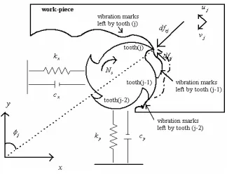
A model, which represents the dynamic compliance between the tool and work-piece in milling processes, has been developed. In this case, it is predicted with analytical methods. The model assumes the cutter to have two orthogonal degrees of freedom and the work-piece to be rigid.

2.1.Dynamic model

The dynamic model of the milling cutter is assumed to be a system with one mode of vibration in each direction, x and y , while the feed direction is along the

x- axis. The milling system under consideration is

shown in figure 1. The milling cutter has ntteeth, which

are equally spaced. The dynamics of the system is given by the differential equations [8],

( )

( )

0

t

n

x x x xj x

j

m x c x k x⋅⋅ ⋅ f t f t =

⋅ + ⋅ + ⋅ =

∑

= (1)

( )

( )

0

t

n

y y y yj y

j

m y c y k y⋅⋅ ⋅ f t f t =

⋅ + ⋅ + ⋅ =

∑

= (2)

where mi, ci and ki are the mass, damping and

stiffness of the tool, fxjand fyj are the components of

the cutting force that is applied by the _jth_{tooth, which}

are obtained by projecting f into the two orthogonal

axis.

2.2.Cutting force model

A simple model of the cutting forces will be discussed here which express the tangential cutting force to be proportional with the instantaneous chip thickness. Despite this simplicity, this model captures the essence of the process. Hence,

t t

f = ⋅ ⋅k b h (3)

where kt is the specific cutting force parameter, bis the

axial depth of cut and h is the instantaneous chip thickness. In addition, the radial force may also be expressed in terms of the tangential force as,

r r t

f =k f⋅ (4)

where kris a proportional constant. This cutting force

model has been used by several authors [6].

The most critical variable in (3) is the chip thickness because it changes not only with the geometry of cutting tool and cutting parameters, but also with the uneven surface left by the previous passes of the cutting tool.

This process is known as regenerative mechanism [6].

The chip thickness is measured in the radial direction, with the coordinate transformation,

sin cos

j x j y j

ν = − ⋅ φ − ⋅ φ (5)

where φj is the instantaneous angular immersion of

tooth j measured clockwise from the normal Y axis

(fig.1).

The resulting instantaneous chip thickness consists of

static part st⋅sinφj, attributed to rigid body motion of

the cutter, and a dynamic component caused by the dynamic displacements or vibrations of the tool at the

present, νj , and previous tooth periods, νoj . Then, the

total chip load can be expressed by,

( )

sin

(

o

) ( )

j t j j j j

h φ =_⎣⎡s ⋅ φ + ν −ν _⎦⎤⋅g φ (6)

in the tool rotate angle domain, or

( )

( )

( ) ( )

( )

(

)

sinsin

( ) (

sin

)

cos

( )

cos

j t j j j

j j

h t s x t t y t t

x t T t y t T t

φ φ φ

φ φ

⎡ ⎤

= ⋅ +_⎣ ⋅ + ⋅ _⎦

⎡ ⎤

−_⎣ − ⋅ + − ⋅ _⎦ (7)

in the time domain, where g

( )

φj is a unit step function

which determines whether the tooth is in or out of cut, st

is the feed rate per tooth, T is the tooth period and, if

the spindle rotates at

(

1

)

s

N rad s_⋅ − _{, the immersion angle}

varies as φj

( )

t =N ts⋅ , and φj

( )

t =0if the j-tooth is

not engaged with the part[6].

2.3.Time domain simulation

Since the system is excited by cutting forces that can not be expressed by simple analytic functions, the equations can not be integrated in a closed form. Hence,

the 4 order Runge-Kutta method is employed to solve th

the differential equations (1) and (2)[8]. A simulation system, which reads the input data of cutting conditions, machine tool characteristics, and other related parameters, and outputs the forces and vibration displacements of chatter in milling has been developed.

2.4.Stability lobes

Projecting ftj and frj determined by equations (3)

and (4) into x and y axis, taking into account that the static component of the chip thickness is dropped from the expression (6), and summing for all teeth engaged and rearranging the above expressions (3) and (4) in matrix form, will yield to [2]:

1 2

x xx xy

t

y yx yy

f a a x

bk

f a a y

∆

⎧ ⎫ ⎡ ⎤ ⎧ ⎫

⎪ ⎪ =

⎨ ⎬ ⎢ _{⎥ ∆}⎨ ⎬

⎪ ⎪ ⎩ ⎭

⎩ ⎭ ⎣ ⎦ (8)

where

a

xx

,

a

xy

,

a

yx

,

a

yycan be easily obtained, and [image:3.612.99.261.76.200.2]

they are angular position dependent.

Considering that the angular position of the parameters changes with time and angular velocity, equation (8) can be expressed in time domain in a matrix form as:

( )

{

( )

}

1 2

x t y

f

bk A t r t f

⎧ ⎫

⎪ ⎪ = ⎡ ⎤ ∆

⎨ ⎬ ⎣ ⎦

⎪ ⎪

⎩ ⎭ (9)

where

{

∆r t

( )

}

=

(

x t

( ) (

−x t T y t−

) ( ) (

, −y t T−

)

)

. The time directional dynamic milling force

coefficients collected in A

( )

t are periodic function of

the tooth passing period,T. Furthermore,A

( )

t can be

expanded into a Fourier series. For the most simplistic approximation, the average component of the Fourier series expansion can be considered. The dynamic milling expression for milling force will be reduced to:

( )

1

[ ]

{

( )

}

2 t o

f t = b k A⋅ ∆r t (10)

where

[ ]

o xx xy

yx yy

A = ⎢⎡α_α α_α ⎤⎥

⎣ ⎦ is the time-invariant but

immersion-dependent directional cutting coefficient matrix [6].

Thus, being ⎡_⎣φ ω

( )

i ⎤_⎦ the transfer function matrix at

the cutter contact zone, denoted by

( )

xx

( )

( )

xy

( )

( )

yx yy

i i

i

i i

φ ω φ ω

φ ω

φ ω φ ω

⎛ ⎞

=

⎡ ⎤ ⎜ ⎟

⎣ ⎦ ⎜_⎝ ⎟_⎠. Furthermore,

describing the vibrations at the chatter frequency, ωc, in

the frequency domain using harmonic functions,

( )

{

}

( ) { }

i tc

c

r iω = ⎡_⎣φ ωi _⎦⎤ f eω ,

{

( )

}

i Tc

{

( )

}

o c c

r iω ₌e−ω r iω _,

( )

{

∆r iωc

}

=

{

r i

( )

ωc

}

−

{

r io

( )

ωc

}

then, the equation (10) can be written as:

{ }

1 1

[ ]

( ) { }

2

c c c

i t i T i t

t o c

f eω ₌ bk _{⎡ −}e−ω _⎤ A _⎡φ ωi _⎤ f eω

⎣ ⎦

⎣ ⎦ (11)

Obtaining the characteristic equation and its

eigenvalue,Λ:

(

1

)

4

c

i t t

N

bk e ω

π

−

Λ = − − (12)

For the case that the cross transfer functions of the systems are neglected, the characteristic equation will be

reduced to a quadratic equation, and the eigenvalues Λ

can be obtained [6].

The critical axial depth of cut is calculated by substituting the obtained eigenvalue into equation (12):

(

2

)

lim

2 1

R t

b

Nk

π κ Λ

= − + (13)

where κ=ΛI ΛR is the division between the

imaginary and real parts of the eigenvalue Λ.

Corresponding to the spindle speed Ns=60 N⋅T

(14) and the chatter frequency can be found [6] as: 2

cT k

ω = +ε π, whereε π= −2ϕ, and _ϕ=tan−1_κ.

T is the spindle period, and kis the integer number

of full vibration waves (i.e lobes), imprinted on the cut arc. The lobes are calculated, selecting a chatter frequency from transfer functions around a dominant

mode, solving the eigenvalue equation(12), calculating the critical depth of cut from (13), calculating the spindle speed from (14) for each stability lobes, and repeating the procedure by scanning the chatter frequencies around all dominant modes of the structure [6].

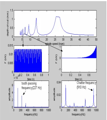
Figure 2 shows, the lobes char, and the analytical time and frequency domain response for a tool 2 system, which characteristics can be seen in section 5. The chatter stability lobes make up a spindle speed (frequency) dependent dividing line between stable (down part line) and unstable (up part line) depth of cut for a certain width of cut. Stable state corresponded figures present a delimit time response, and the tooth passing frequency and its harmonics, frequency response. Unstable state corresponded figures present a not delimit time response, and the chatter frequency is appreciated.

3.

Expert system

The main objective of the expert system is to obtain a mill cutter, among the available ones, which have an operating point or adequate cutting parameters, with acceptable productivity (MRR), robustness stability against spindle speed perturbations and less power consumption than the spindle motor availability.

For this purpose, it is got the allowable cutting space parameter, spindle speed, feed rate and axial depth of cut for a constant radial depth of cut, taking into account the regenerative chatter instability and the power available in the spindle motor. Then, a novel cost function is schemed. It is inversely proportional to MRR and a parameter determinate as stability against spindle speed perturbation, and proportional to power consumption. Each term of the cost function have a proportionally

[image:4.612.324.512.127.339.2]

factor to have terms of the same magnitude. Also, there is a weight factor which measures the importance of each term. The weight factors are intended to be programmed by the machine operator.

3.1.Milling process determination and preliminary rules

In order to evaluate the system performance, it is needed to select a suitable tool and performance indices. Milling processes, basically, consists of two phases roughing and finishing the surface. The main difference between these operations is to decide the most appropriate performance index for a given tool. The quality and geometric profile of the cutting surface is of paramount importance in milling finishing operation, whereas roughing -milling consists on removing a large amount of material from a blank.

This paper deals with roughing milling operation. The rate at which the material is removed is called material removing rate (MRR). This parameter measures the productivity of machining processes. In milling operations, MRR is defined as the multiplication between axial and radial depth of cut, and feed per tooth. MRR upper limit, is given by, chatter vibrations and power deliver by the spindle motor. At certain combinations of cutting parameters, such as spindle speed, axial depth of cut and feed per tooth, either chatter vibrations are appreciate, or the power available by the spindle motor is insufficient. Then, these parameters bound the roughing milling productivity.

For those reasons, at a first approximation, the input cutting parameter space is given by the cutting parameters, which are below the line at the stability lobes char, and the power consumption is less than the power available by the spindle motor.

But, due to the approximations in constructing stability chars, the lobes are constructed, not by replacing pure imaginary roots into the characteristic equation, but adding a positive real number to them. Furthermore, to have a robust system, it has been taken into account a confine in a programmed maximum depth of cut.

Then, the following algorithmic methodologies are

used, which are called preliminary rules:

• Rule1: Stability margin setting to ensure that the system plays in a stable region, despite the system model uncertainties.

• Rule 1.1: For calculating secure stability lobes char, a small stability margin is selected, i.e, it is supposed that the chatter vibrations happen at

c

i⋅ω +

δ instead of at i⋅ω_c. The reason is that

the stability border line is calculated from a

linear approximation. Then, i⋅ω_c is replaced

by δ+i⋅ω_c,δ>0, when the stability border

line is calculated. This rule is applied to the equation (13).

• Rule 1.2: For improving the robustness of the system, it has been taken into account a margin at the final expression for chatter free axial depth of cut, equation (18), i.e,

1 0 , b

b_lim =α⋅ _lim <α< . This rule lets a better

control capacity in the spindle speed. On the other hand, a better MRR selection is lost.

• Rule 2: For searching the allowable input space parameter, the set of spindle speed, Ns, axial depth

of cut, b and feed rate,st.

• Rule 2.1: Calculate the boundary points, spindle speed and axial depth of cut pairs, which compose the line between stable and unstable zones, satisfying Rule 1. This rule is obtained by plotting the stability lobes char, which gives the line between stable and unstable zones

• Rule 2.2: Calculate the admissible input space, )

s , b , N ( :

Q = _{s t} . The boundaries spindle speed

and axial depth of cut, gives the maximum spindle speed and axial depth of cut pairs without chatter vibrations (rule 2.1). The time domain simulations output the system dynamical force shape. As it will be seen in the next section, the spindle power is force dependent, which is spindle speed, axial depth of cut and feed rate dependent. Then, for a given spindle motor power available, the

admissible input cutting parameter space is

obtained.

3.2.Tool selection

In this section, an approach for tool selection is suggested. For this purpose, a tool cost model function is designed. The designed tool cost model is used to select the appropriate tool between the candidates though the optimisation Rules, explained below.

Then, the study requires a given set of candidates milling cutters. Each one is characterised by the following properties:

(

, , , , , , , ,

)

i nxi nyi xi yi xi yi ti i i

R = ω ω ξ ξ k k n D β where,

(

ω ω ∈xi, yi

)

W is the tool natural frequency,

(

ξ ξxi, yi

)

∈ξ is the tool damping ratio,

(

k kxi, yi

)

∈K is

the tool static stiffness, nti is the tool number of teeth,

i

D is the tool diameter and βiis the tool helix angle.

i

R∈T, i=1, 2,..,N, where N is the number of tools and

T is the set of tools available to the designer. W is the

set of tools’ natural frequencies, conformed by the pairs

(

ω ωx, y

)

for each tool, ξ is the set of tools’ damping

ratio, conformed by the pairs

(

ξ ξx, y

)

for each tool and

tools’ static stiffness is conformed by

(

k kx, y

)

for each

tool.

3.2.1.Tool cost model definition

model for a single milling process can be calculated using the equation (20).

(

1 2

)

1 1

3 2

2 3

, , ; , ,

t s t

s

C P MRR N R c c c NF P NF

NF

c _MRR c _N

∆ = ⋅ ⋅

+ ⋅ + ⋅ _∆ (20)

with 3

1 1 i i c = =

∑

, R T∈ , where

( )

1

t

n t tj j

j

P V f φ

=

= ⋅

∑

,

t

MRR a b s= ⋅ ⋅ , ∆Ns takes its definition given below,

and q≡

(

N b ss, , t

)

∈Q. Standardizing factors, NFi, are

defined as follow, 1

1 tAv

NF ₌P − _{, where}

tAv

P is the power

available in the spindle motor, NF2=MRRmax, where

max

MRR is the maximum MRR with the chatter vibration

and spindle power restrictions calculated among all the

candidate cutters and NF3= ∆Nmax, where ∆Nsmaxis the

maximum measured value of this variable among the candidate cutters.

The tool cost function is designed to be MRR, power consumption, and a range against possible perturbations in tool rotational motion, dependent and inversely proportional to MRR and a range against possible perturbations and directly to power consumption.

These parameters have the following definitions:

Material or Metal Removing Rate

(

MRR

)

t

s b a

MRR= ⋅ ⋅ , where, a is the radial depth of cut, b is

the axial depth of cut and s is the linear feed rate. The t

MRR is a parameter, which compares, the efficiency of the milling process. A larger MRR improves the process productivity.

Cutting power draw from the spindle motor

( )

Pt

The cutting power, P_t, drawn from the spindle motor

is found from,

( )

1

t

n t tj j

j

P V f φ

=

= ⋅

∑

(21)

whereV=π⋅D⋅N_sis the cutting speed and N_s is the

spindle speed. The tangential cutting force is given by:

( )

( )

tj j t j

f φ =K b h⋅ ⋅ φ (22)

where b is the axial depth of cut, K_tis the cutting force

coefficient, which are material dependent and is

evaluated from experiments, and h

( )

φi is the chip

thickness variation, which is feed rate st (mm/rev-tooth)

dependent.

Spindle speed security change

(

∆Ns

)

An additional term, spindle speed security change, is added to the cost function model to be sure that chatter vibrations are avoided. The spindle speed security

change, ∆N_s, measure the nearest spindle speed at

which chatter vibrations happen to the supposed spindle speed it will be operated. This fact allows to have an error margin due to possible perturbations in this variable.

To calculate analytically,∆Ns, the following

algorithmic methodologies are carried out. They are divided in two cases:

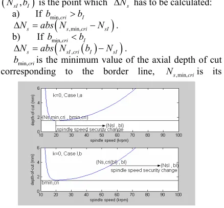
Case I: k=0, this case corresponds to pairs, spindle

speed, axial depth of cut, situated below the first lobe of the stability chars. Then, there is no lobe in the right part

of the point as it can be shown in figure 3. Suppose that

(

N bsI, I

)

is the point which ∆Ns has to be calculated:

a) If bmin,cri >bI

(

,min,

)

s s cri sI

N abs N N

∆ = − .

b) If bmin,cri<bI

( )

(

,

)

s sI cri I sI

N abs N b N

∆ = − .

min,cri

b is the minimum value of the axial depth of cut

corresponding to the border line, Ns,min,criis its

corresponding spindle speed, Ns cri,

( )

bI is the

left-projection of the point

(

N bsI, I

)

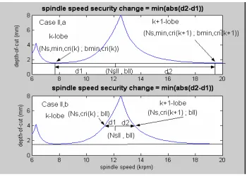
into the nearest lobe.

Case II: k≠0, in this case, the point ,which ∆Ns has

to be calculated, is situated between two lobes in the

stable region. Suppose that

(

NsII,bII

)

is the mentioned

point, then ∃k such

thatNs,min,cri

( )

k <NsII<Ns,min,cri

(

k+1

)

, where kis the

lobe number, k=0,1..S−1, and S is the number of

printed lobes , and Ns,min,cri

( )

k is the spindle speed

corresponding to the axial depth of cut minimum value

on the border line, bmin,cri

( )

k , for the k-lobe. Then:

a) If bmin,cri

( )

k > <b bmin,cri

(

k+1

)

( )

(

)

(

)

(

,min,,min,

)

, min

1

s cri s s

s cri s

abs N k N

N

abs N k N

⎛ − ⎞

∆ = ⎜_{⎜ + −} ⎟_⎟

⎝ ⎠

b) If bmin,cri

( )

k < >b bmin,cri

(

k+1

)

( )

(

)

(

)

(

,,

)

, min 1

s cri s s

s cri s

abs N k N

N

abs N k N

⎛ − ⎞

∆ = ⎜_{⎜ + −} ⎟_⎟

⎝ ⎠

whereNs cri,

( )

k is the left-projection of the point

(

NsII,bII

)

into the k-lobe, and Ns cri,

(

k+1

)

is the

right-projection into the k+1-lobe. The case under consideration is graphically represented in figure 4.

Note that, standardization factors,NFi, are also added

to the cost function to have terms with the same magnitude. Moreover, they make to have a relative term between all the candidates cutters involved. On the other hand, these terms ensure that the cost function will be comparable among the different cutters.

The ,c ii =1,..,3, values are the weights of the cost

function terms. They measure the importance of the cost function terms. The below optimisation Rule 3 give a

[image:6.612.316.535.82.286.2]

pattern to program the ci.

3.2.2.Optimisation Rules

The above defined tool cost function is used to select the appropriate tool and cutting parameters, through the following optimisation rules.

Rule 3 : Weight factors selection

The weight factors are intended to be programmed by the machine operator. An extended explanation of their meaning and their adequate selection is given in this

section To select suitable values of ci, i=1,..,3, their

meaning has to be perceived. The c1, measures the

importance of the spindle power consumption. The

larger c1 parameter is the more important to the spindle

power consumption in the cost model function. The

2

c measures the machine productivity, if the c2is near to

one high productivity is required, and if it is near to zero the productivity has no importance. The same reasoning

is applied to the c3, which measures the stability against

possible perturbations in the spindle speed variable. It has to take into account that the expert system, ensures that the spindle power consumption is always going to be smaller than the power available in the spindle motor, through Rule 1. Also, that the cutting parameter space has no problems due to chatter vibrations through Rule 2.

Then, a possible criterion leading to a process with acceptable productivity, which is the main objective of

the milling processes, c2about 0.75, and the other two

constants will add 0.25 , suitable values are c1=0.1 and

2 0.15 c = .

Rule 4 : Tool selection criterion

A simple tool selection criterion for cutter selection has been developed. For a given values of c1,c2,c3, and a given tool characteristics, the cost function value is obtained for all the admissible input cutting parameter space. The minimum value of the cost function is saved. The procedure is repeated for all the available cutters. Comparing the minimum value of the cost function for all available or candidate cutters, the corresponding cutter to the minimum value of the minimum value of the cost function is the selected tool.

The selection criterion is, mathematically, expressed as:

• Compute,

( )

( )

( )

(

tj j , j j , sj j ; , ,i 1 2

)

C P q MRR q ∆N q R c c ; (23)

for each Ri∈Ti, i N∈ , and Nis the set of

candidate tools and ∀ ≡qj

(

N b ssj, ,j tj

)

∈Qwhere

{

1,..,

}

p _p

j N∈ = N is a discrete sub-space of the

cutting parameters space where the cost function (20) is calculated.

• For obtaining the selected tool, ST, compute

( )

( )

( )

(

, , ; , ,1 2

)

,

arg min t j j s j i

i N j

C P q MRR q N q R c c ST

q Q

∈

⎧ ⎫

⎪ ∆ ⎪

= ⎨ _∈ ⎬

⎪ ⎪

⎩ ⎭

with ST T∈ , obtaining the appropriate tool according

to the criterion.

Following the rules, the expert system provides an appropriate cutter among the candidates.

Rule 5 : Cutting parameter selection

• Rule 5.1 : General case

To select the cutting parameters, there are two possibilities. First of all, directly, calculate the cutting parameters, which correspond to the selected tool, which gives the minimum value of the cost function. It can be expressed mathematically as,

• Compute the following equation (24)

(

)

( )

( )

( )

(

)

{

}

* * * *

1 2

, ,

arg min , , , , ,

j

s t

t j j s j

q Q

q N b s

C P q MRR q N q ST c c

∈

≡ =

∆

obtaining an input cutting parameter for the selected tool.

The cutting parameter space is obtained by checking all possible values of spindle speed and axial depth of cut which are below the stability line in the stability char according to Rule 1. These values join to the allowable feed rates, which do not make consume more spindle power than the available, Rule 2, form the cutting parameter space. For the selected tool, the trio of cutting parameters which minimize the cost function are, then, selected.

• Rule 5.2 : Refinement case

In order to have a more accurate possibility, it has been taken into consideration that the cutting parameters can be searched with a more fine integration step around the point where the cost function gives its minimum value. Now, the cutting parameter space is given by a

3-tuple

(

( )* ( )* ( )*

)

* k , k , k

s t

Q = N b s around _q*_{, for k=1,..,p, where}

p is the number of points to be considered, according to Rules 1 and 2. The procedure for obtaining the required cutting parameter is the same as used in Rule 5.1 trough equation (24) for the above defined new cutting parameters.

Mathematically expressed :

• Compute

( )

( )

( )

( )

( )

( )

( )

(

)

{

}

*

* * *

**

1 2 *

arg min_k k , k , k , , ,

t s

q Q

q C P q MRR q N q ST c c

∈

= ∆

[image:7.612.91.266.74.199.2]

Obtaining the refined cutting parameter.

Rule 6 : Process malfunctions : tuning c c c1, ,2 3values

Nevertheless, in programming the selected tool and cutting parameters, malfunctions of the process may lead to a poor behaviour of the process. The most important are tool wear and burr formation. These phenomena, which are common in the manufacturing processes, make that the analytical and experimental testes are not always in concordance. If it is happened, the follow algorithmic methodology could be applied:

While

chatter toothpast

A >A

2 0.99 2

c ← ⋅c

3 0.01 1 3

c ← ⋅ +c c end

where Achatter is the chatter frequency vibration amplitude,

and Atoothpastis the highest amplitude among the tooth

passing frequency and its harmonics. So, a more stable state is obtained.

Finally, figure 5 shows a scheme of the expert system.

The developed expert system takes the α and δ

constants, the tools´ modal parameters such as its natural frequency, damping ratio, tool static stiffness, number of teeth, the radius of the tool, the helix angle, and the cutting constants for the work material and cutter (tools´ characteristics), the spindle power available and the cost function weight factors, as inputs and outputs the appropriate tool among the candidates and robust programmed cutting parameters.

4.

Example

For the validation of this method, the above study has been applied for two practical straight cutters and a full-immersion up-milling operation. The example considers the tools to have the following characteristics, according with the section 3.2 notation,

(

)

1 603, 666,3.9,3.5,5.59,5.715,3,30,0

R = , and

(

)

2 900.03,911.65,1.39,1.38,0.879,0.971, 2,12.7,0

R = .

The natural frequency is measured in hertz, the tool

damping is in %, the tool stiffness is in _{KN mm⋅} −1 _and

the diameter of the tool is in mm. The work-piece is a

rigid aluminium block whose specific cutting energy is

chosen to be 2

^ 1,2t 600

k ₌ kN mm_⋅ − _{and the proportionally}

factor is taken to be kr1=0.3, for the tool one, and

2 0.07 r

k = for the other one. Other expert system

parameters are, the stability margin factor, δ =0.05and

the stability margin factor for the axial depth of cut, 0.95

α = .

The analytical test for mill cutter selection was conducted using spindle speeds with increments of

1000rpm, axial cutting depth started with its minimum

value in the stability border line divided by ten, and it is increased in steps of this same size, for a given spindle speed. The operation constrain on the maximum feed per

tooth is 0.55mmand the step integration is taken to be

0.05. The spindle power availability is 745.3W.

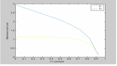
The resultant tool is that leading to the minimum tool cost function value. In figure 6, it is shown the values of

tool cost function as c1parameter varies, the c3has been

taken as a constant c3=0.075and the c2 follow the rule

2 1 1 2

c = − −c c . This study has been done to illustrate the

influence of the ciparameters in the tool cost function. It

is observed the tool R1has a better behaviour respect to

the tool R2for all possible value of c1and c2, with

3 0.075

c = . Analysis with other values of c c1, 2 and c3,

have been carried out and the results are similar, and the

tool R1 has a better behaviour. Then, a more general

analysis shows in figure 7, in which the minimum value of the tool cost function for all possible combinations of

1, ,2 3

c c c , with the restriction c1+ +c2 c3=1is displayed.

[image:8.612.323.521.240.353.2]

The analysis has revealed that the first tool has a better

Figure 6: Minimum-C function vs. c1varies, with c3 =0.075.

[image:8.612.93.504.544.700.2]

behaviour than the second one for all combinations of

the ciparameters. Thus the output of the expert system is

the first tool.

For the cutting parameters selection, two steps have been done. First, the cutting parameter corresponding to the minimum of the tool cost function for the selected

tool for values of c1=0.2,c2=0.725,c3=0.075is

obtained. These values are _q*_{=(5800, 0.4924,0.2722).}

It can be a well-done first approximation. For a more accurate solution, the tool cost function is evaluate around the above mentioned cutting parameters. Then,

another integration is taken into account around _q*_{. The}

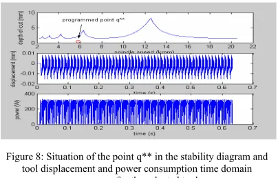
[image:9.612.85.292.106.214.2]

test for cutting parameters selection is conducted using spindle speeds between 5700 and 5900 rpm, and a step of 20, axial depth of cut between 0.48 and 0.52 and a step of 0.01, and the feed per tooth between 0.25 and 0.35 and a step of 0.025. The resulted programmed cutting parameters are_q** ₌

(

5780,0.494,0.28

)

_.

Figure 8 shows the situation in the stability lobes of

the programmed point q**, the tool displacement and

the power consumption. It is observed that the point is robustly stable and the power consumption is less than the power availability in the spindle motor, while acceptable MRR.

This method can be applied to any number of selected tools generating in a automatic task the best one to be used in the system. Moreover, the method can be used to schedule the relative compliance between the available tools and the used work-pieces materials. Finally, the expert system can be used to optimise the manufacturing process, in the sense of planning the adequate sequence

of work-pieces to be manufactured for each tool in order to minimise the changes of tools.

5.

Conclusion

An efficient approach for mill cutter selection has been developed through an expert system. The expert system is instructed with the characteristics of the candidates tools, as well as with the stability margin and constrains of operations, such as, power availability and robust. Furthermore, a tool cost model function, built from the expert systems preliminary rules, is proposed to evaluate the possible performance of each candidate tool in milling process. This performance index is then used to select an appropriate tool and cutting parameters for the operation which lead to the maximum productivity, while respecting stability and power consumptions margins though optimisation rules. A simulation example which shows the behaviour of the system is presented.

Acknowledgements

The Authors are very grateful to MCYT by its partial support through grant 2003-00164 and to the UPV/EHU through Project 9/UPV 00I06.I06-15263/2003.

References

[1] S. Y. Liang, R. L. Hecker and R. G. Landers, “Machining Process Monitoring and Control: The State of the Art”, Journal of Manufacturing Science and Engineering, Vol.126, pp. 297-310, 2004.

[2] S. V. Wong and A. M. S. Hamouda, “The development of an online knowledge-based expert system for machinability data selection”, Knowledge-Based Systems, Vol.16, pp. 215-219, 2003.

[3] M. C. Cakir, O. Irfan and K. Cavdar, “An expert system for die and mold making operations”, Robotics and Computer-Integrated Manufacturing, Vol.21, pp. 175-183, 2005. [4] A. Vidal, M. Alberti, J.Ciurana and M. Casadesús, “A decision

support system for optimizing the selection of parameters when planning milling operations”, International Journal of Machine Tools and Manufacture, Vol.45, pp. 201-210, 2005.

[5] I. D. Carpenter and P. G. Maropoulos, “A flexible tool selection decision support system for milling operations”, Journal of Materials Processing Technology, Vol.107, pp. 143-152, 2000. [6] Y. Altintas, Manufacturing Automation, Cambridge University

Press, 2000.

[7] O. Maeda, Y. Cao and Y. Altintas, “Expert spindle design system”, International Journal of Machine Tools and Manufacture, Vol.45, pp. 537-548, 2005.

[image:9.612.88.290.404.533.2]

[8] L.Rubio and M. De la Sen, “Analytical procedure for chatter in milling”, Southeastem Europe, USA, Japan and European Community Workshop on Reseach and Education in Control and Signal Processing, June 14-16, 2004, Cavtat, Croatia Figure 7: Minimum-C function versus c1,c2,c3varies.

Figure 8: Situation of the point q** in the stability diagram and tool displacement and power consumption time domain