Mian, Naeem S., Fletcher, Simon, Longstaff, Andrew P., Myers, Alan and Pislaru, Crinela
Novel and efficient thermal error reduction strategy for machine tool performance improvement
Original Citation
Mian, Naeem S., Fletcher, Simon, Longstaff, Andrew P., Myers, Alan and Pislaru, Crinela (2008)
Novel and efficient thermal error reduction strategy for machine tool performance improvement. In:
Proceedings of Computing and Engineering Annual Researchers' Conference 2008: CEARC’08.
University of Huddersfield, Huddersfield, pp. 1522. ISBN 9781862180673
This version is available at http://eprints.hud.ac.uk/id/eprint/3673/
The University Repository is a digital collection of the research output of the
University, available on Open Access. Copyright and Moral Rights for the items
on this site are retained by the individual author and/or other copyright owners.
Users may access full items free of charge; copies of full text items generally
can be reproduced, displayed or performed and given to third parties in any
format or medium for personal research or study, educational or notforprofit
purposes without prior permission or charge, provided:
•
The authors, title and full bibliographic details is credited in any copy;
•
A hyperlink and/or URL is included for the original metadata page; and
•
The content is not changed in any way.
For more information, including our policy and submission procedure, please
contact the Repository Team at: [email protected].
NOVEL AND EFFICIENT THERMAL ERROR REDUCTION STRATEGY
FOR MACHINE TOOL PERFORMANCE IMPROVEMENT
N. S. Mian1, S. Fletcher 1, A. P. Longstaff 1, A. Myers 1, C. Pislaru 1
1
University of Huddersfield, Queensgate, Huddersfield HD1 3DH, UK
ABSTRACT
The accuracy of a machine tool is affected by the heat generated during the machining process. Also, varying environmental conditions produce thermal gradients that flow through the machine structure. The heat passes through assembly joints and structural linkages in the machine where the roughness and form of the contacting surfaces affects the heat transfer coefficients. Measurement of the thermal behaviour and associated deformations in the structure is a time consuming procedure where machine downtime is a dominant issue. This paper discusses a novel offline technique using Finite Element Analysis (FEA) to simulate the thermal distribution and deformations during the spindle heating and cooling cycle in static conditions on a small Vertical Machining Centre (VMC) CNC machine. Detailed experimental testing of the temperature distribution in the machine and heat transfer work to obtain accurate values of the thermal contact resistance across the joints is reported. The obtained experimental results are evaluated and applied to the FEA software to obtain thermal distribution and associated deformations in a machine tool structure offline. The FEA simulated results are presented and are in close correlation with the obtained experimental results. FEA simulation enables efficient offline assessments of temperature distribution and displacements in the machine tool structures that result in a significant reduction in machine non-productive downtime while enabling characterisation under variable environmental conditions.
Keywords: Finite element analysis, FEA, Thermal error, Thermal deformations, Machine tool accuracy
1 INTRODUCTION
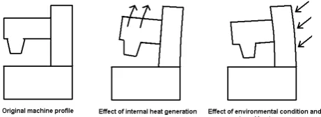
The accuracy of machine tools is largely influenced by the positioning error that produces deviations in the movement of the machine parts. Thermal error can represent 70% of the total positioning error, (Bryan (1990)), which is a combination of machine tool’s internal heat and the environmental changes. The continuous usage of a machine tool causes heat to generate which leads to thermal error distorting the accuracy due to thermal expansions of structural linkages; this is considered as a major issue in engineering industries due to high demand of micron precision in the produced parts. Environmental swings also play a major contribution in the generation of thermal error that affects the machine transiently during the day and night, (Longstaff (2003)). Figure 1 shows the general effect of internal heat and environmental conditions on a machine tool. Major possible machine tool internal heat sources can be classified as installed motors, spindle bearings, gears, clutches, hydraulic oil, pumps belt drives, and axes ball screws. The heat enters into machine’s discrete structure and passes through mechanical joints which exhibit a non linear thermo-elastic behaviour depending upon the material properties of structural joints and their contact roughness accuracy. (Ramesh (2000)).
Thermal non linear behaviour across joints depends on various contact properties which are discussed in detail in section 2. Uniqueness of these contact properties is considered as a major issue in FEA modelling. A great deal of suitable information is available for thermal contact resistance values, (Janna and Heikal (1988)), but those are generic values where precision parameters in contact properties are not highly considered. Series of experiments were conducted to obtain accurate thermal contact resistance values across the joints and high importance was given to represent the real world machine tool assembly joints to obtain accurate results from FEA simulations.
Abaqus CAE 6.7-1 (Dassault Systemes (2007)) software is used to create models of machine tool spindle, carrier, tool and column for FEA due to its ability to develop user programmable subroutines to describe varying spatial boundary conditions representing varying environmental conditions and ability to handle complex geometrical structures and assemblies.
static thermal deformations. This paper will detail the experimental work carried out to obtain relevant data for offline simulations of the thermal behaviour in the machine tool.
2 THERMAL CONTACT RESISTANCE TESTING
In order to obtain the internal thermal distribution in the machine which is a resultant of the internal generated heat flowing through structural joints, it was important to evaluate thermal contact resistance at the contacting surface which controls the heat flow across joints.
2.1 Thermal contact resistance and behaviour
Thermal contact resistance (TCR) across the joints produces a temperature drop which depends on local contact configurations such as contact pressure, number of contact points, size and shape of contact points, size of voids, type of fluid in voids, pressure of fluids in voids, hardness of contact surfaces, flatness of contacting surfaces, modulus of elasticity of contact surfaces, average surface of contacting surfaces and surface cleanliness. Figure 2 shows an overview of the thermal resistance across the joint (Hagen (1999)). Since conduction is the only significant method of heat transfer across mating points in the joint, the non linear behaviour at the structural joints is due to the fact that the rest of the heat transfer is controlled by the contact configuration, the thickness of the interfacial gap and the thickness of the surface film and all these depend on the local contact pressure. When there is a change in a local contact configuration, there is change in the interfacial gap that causes a change in the surface film and in turn causes a variation in the heat flux. The resulting heat flux generates thermal contact stresses that alter the existing pressure distribution. This is repeated until a state of equilibrium is achieved. This theory explains the fact that the distribution of the contact pressure along the joint controls the transfer of heat from one structural element to another which in turn results in non uniform deformations of structural elements due to non uniformity in the values of thermal contact resistance. (Ramesh (2000))
2.2 Testing:
High importance has been given to the surface finish, surface flatness and cleanliness of the components to replicate the precision and accuracy used in assembly of the machine tool.
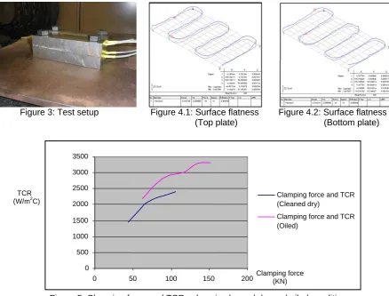
Experiments were carried out on two rectangular steel plates with average surface finish of 3 microns and surface flatness of 14 microns. Four digital thermal sensors were placed in both plates. Figure 3 shows the test setup and Figure 4.1 and Figure 4.2 show the surface flatness of both plates measured by a Ziess Coordinate Measuring Machine (CMM).
Prior to the TCR experiments, it was important to obtain the convective heat transfer coefficient or heat loss to the air during heating and cooling phases of the body. This has influence on the surface of the body and results in decreasing the surface temperature. In order to obtain the convection coefficient value, one of the steel plates was heated up to 50˚C and suspended in air to cool down at room temperature of 25˚C in a free convection mode. The convection value obtained was 8W/m2C which was calculated from equation 1.
T
hA
Q
=
Δ
(1)Where h is the convection coefficient for air, A is the area of plates and
Δ
T
is the temperature difference between the starting the heated cycle temperatures. After quantifying the convection coefficient, TCR experiments were carried out in two phases, firstly with cleaned dry plates and the second with oiled plates. In the first phase, plate-1 was heated up to approximately 52˚C and plate-2 placed immediately and fastened onto the heated plate-1 using four bolts. Contact pressure at the joint was varied by using torque values ranging from 35Nm to 85Nm applied to the fastening bolts (M14) to evaluate the effect of increasing contact pressure or clamping force on the TCR value across the joint. The heat energy flowing through first plate to the second with the convection also taking place is calculated from equation 2.T
hA
T
mCp
Q
=
Δ
+
Δ
(2)Pi = T/ (KD) (3)
Where Pi is the clamping force, T is the toque applied, K is the torque coefficient and D is the bolt nominal diameter.
In phase 2, the same test was repeated by applying oil on the plate’s contacting surfaces, to change the condition of the plates from dry to wet or from clean to dirty. An increased trend of TCR was observed from dry to oiled conditions. Chart 1 illustrates the values obtained in dry conditions and oiled conditions for TCR values and the clamping forces across the joint. The values obtained were applied to the FEA models to accurately predict the thermal behaviour over the structure. Figure 5 shows the clamping force and TCR profiles in dry cleaned and oiled conditions. An increased proportion of TCR with increasing torque can be observed.
Torque Clamping forces Pi (KN) for four M14 bolts
TCR values (W/m2C)
T cleaned dry Oiled cleaned dry Oiled
35Nm 43.54 62.44 1452 2172
45Nm 55.98 80.28 1757 2653
55Nm 68.42 98.12 2064 2920
65Nm 80.86 115.96 2209 3009
75Nm 93.30 133.80 2304 3288
85Nm 105.74 151.64 2402 3315
Chart 1: Experimental values for clamping forces and TCR values at different torque ranges
As the spindle is clamped to the carrier using torque of 70Nm (from manufacturer spindle diagram) to 6 bolts, the clamping force calculated was 129KN which can be used to estimate TCR obtained with the clamping force of 105.74KN at torque value of 85Nm. The TCR value between both contacting surfaces can be estimated to 2500 W/m2C to simulate the heat flow across spindle carrier contact.
Oil lubricated angular contact ball bearings are fitted in the spindle for tool rotation and the TCR value can be taken as 2172 W/m2C representing 36Nm torque applied to the bearing caps. (From manufacturer spindle diagram).
3 ABAQUS MODELS:
For quick and optimised analysis, idealised models of the spindle, carrier, tool and column of a small VMC CNC machine were created in Abaqus 6.7-1. Idealisation features include symmetry constraints applied on symmetrical nature of the spindle, carrier, tool and the column structure over X axis. Figure 6 shows the created and assembled model. Bearings, belt drives and motor supporting structure were simplified and represented as heat generation sources in the machine CAD model.
4 MACHINE TOOL TESTING
As explained previously, continuous usage of machine tool generates heat. The rate of heat generation varies depending upon various factors in general such as spindle speed, movement and rotation feed rates, cutting loads, cutting depths and material properties of the work piece and machine structure. Taking above into account the spindle was rotated at fixed speed of 4000rpm and at constant feed rate during machine testing for heat generation consistency. At this stage it was important to calculate the convective heat transfer coefficient due to increased airflow across the spindle. The test for convective heat loss (section 2.2) was repeated again with the fan placed about a meter distance from the suspended heated plate blowing air with air flow replicating to the flow of air across the rotating spindle at 4000rpm. The value obtained was 35 W/m2C which can be used to simulate thermal distribution across the spindle.
4.1 Thermal testing
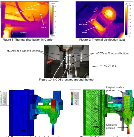
comparison with the obtained simulated temperature profiles. Figure 8 shows the thermal image illustrating thermal distribution in the structure. Figure 9 shows the thermal image taken above the machine and shows the thermal ranges and distribution.
4.2 Displacement testing
Five Non Contact Displacement Transducers (NCDTs) were placed around the a test mandrel (see Figure 10) to monitor the displacements in the tool in X, Y and Z axes due to the thermal effect produced by one hour spindle heating and cooling test. Again the displacement values obtained from NCDTs are shown in section 5.3.1 for reviewing them in direct comparison with the obtained simulated displacement results.
5 ABAQUS SIMULATIONS
The thermal information obtained from one hour heating was analysed and applied in the FEA simulation software for offline thermal assessment. The data obtained from experiments was converted into thermal loads for applying as body heat flux generated from the heat sources in the software. This methodology to obtain body heat fluxes has been tested through benchmark tests in Abaqus to simulate heat distribution originating from those complex structures where thermal sensors are found hard to install for e.g. spindle bearing temperature cannot be directly measured therefore the data was obtained using spindle boss sensors and since bearings are the main heat sources in the rotating spindle, this was converted into thermal load and applied as body heat flux generated from the bearings. Similarly the surface temperature information from the carrier sensors and thermal imaging were analysed and converted into body heat fluxes for belt drive and motor housing support structure.
5.1 Calculations
The thermal information obtained from experiments was used to calculate the heat energy produced in structure. The energy required to raise the temperature by certain amount is calculated from equation 4.
T
mCp
Q
=
Δ
(4)As the convection also taking place at the same time and the workshop temperature observed to be similar to the room temperature observed during convective heat loss experiments, convection coefficient values of 8W/m2C (static air across the carrier) and 35W/m2C (air flow around the spindle) could be used to calculate the heat loss during heating cycle from the carrier and the spindle surfaces respectively and added into the obtained total energy of the associated structure. During cooling cycle 8W/m2C was used for the whole machine due to static air around the whole machine structure. The total energy can be calculated using equation (2). The results were then divided by the volume of concerned heat source to obtain body heat flux value to be applied in Abaqus.
5.2 Thermal Simulation
Calculated body heat fluxes were applied as heat generation sources with the simulation set for two hours with one hour heating and followed one hour for cooling. The thermal results were then used to carry out the displacement analysis.
5.2.1 Thermal Simulation Results
Sensors and nodes location Actual temperatures (˚C) Simulated temperatures (˚C)
% correlation between experiments and simulated results
Heating (max) Cooling (min) Heating (max) Cooling (min) Heating (max) Cooling (min)
Spindle boss 29.18 27.68 29.30 27.26 99.6 98.45
Strip 1 (start) 28.06 27.31 27.41 25.96 97.67 95.05 Strip 1 (end) 25.81 26.12 25.87 25.07 99.77 95.9 Strip 2 (start) 26.43 26.81 27.89 26.68 94.5 99.5
Strip 2 (end) 26 26.31 26.92 25.41 96 96.5
Chart 2: Experimental and simulate temperature results during one hour heating and one hour cooling cycle with correlation results.
5.3 Displacement Simulation
One hour heating and one hour cooling simulated temperature information was fed into the displacement model created in Abaqus to observe any displacements i.e. thermal error in the machine structure.
5.3.1 Displacement Simulation Results:
Figure 12 shows the machine behaviour (displacements) due to temperature distribution. Chart 3 below shows the actual and simulated displacement values obtained at the tool during heating and cooling test. As explained in section 5.2.1, the nodes were picked up from the similar physical locations where the NCDTs were placed (see figure 10). Accuracy in the results showed the correlation ranging from 40% to 71% for heating cycle and 40% to 99.6% for cooling cycle. The variations in correlation may be due to the discrepancies between the simulated top (carrier) and bottom (spindle/carrier) temperature gradients which affected the machine structure bending sensitivity.
NCDTs location (see figure 10)
Actual displacements
(microns)
Simulated displacements (microns) at nodes locations
similar to physical NCDTs location
% correlation between experiments and simulated results Heating (max) Cooling (min) Heating (max) Cooling (min) Heating (max) Cooling (min)
X top 4.05 2.44 2.78 2.43 68.64 99.59
X bottom 4.18 1.95 5.87 0.79 59.56 40.5
Y top 18.75 16.8 29.77 10.92 41.22 65
Y bottom 25.25 23.19 32.62 11.46 70.8 49.41
Z 8.30 7.32 11.15 9.4 65.66 71.5
Chart 3: Actual and simulated displacement results during one hour heating and one hour cooling cycle with correlation results.
6 FUTURE WORK
7 CONCLUSIONS
Thermal distribution and its associated error in a small VMC CNC Machine tool was studied and analysed experimentally and predicted offline using FEA technique. Accuracy measures between contacting surfaces in assemblies and structural linkages were given high importance to evaluate values as accurate as possible in order to obtain optimised FEA results. In depth experimental work carried out to obtain the thermal behaviour in the machine structure by running the machine for one hour heating and one hour cooling cycle. The results obtained from experiments were analysed and applied in the FEA simulation software Abaqus 6.7-1. Temperature distribution results from FEA matches very well with the experimental results obtained compared to the displacement analysis. Simulated FEA technique enabled offline assessments of the temperature distribution and displacements in a machine tool and hence played a significant role in reduction of machine tool non productive downtime.
REFERENCES
Bryan J (1990),
International status of thermal error research
, Ann. CIRP, 39, 645-656.
Longstaff AP, Fletcher S and Ford DG (2003), Practical experience of thermal testing with reference to ISO 230 Part 3, Sixth International Conference on Laser Metrology and Machine Performance – LAMDAMAP 2003, University of Huddersfield, pp 473 – 483.
Ramesh R., Mannan M.A, Poo A.N (2000), Error compensation in machine tools – a review Part II: thermal error, International Journal of Machine Tools & Manufacture, v40, pp 1257-1284.
Janna W.S, Heikal M ed. (1988) ‘Engineering heat transfer’ SI edition, Van Nostrand Reinhold (International).
Dassault Systemes 2007, ABAQUS 6.7-1 FEA software, ABAQUS, Inc.
Hagen K.D (1999), Heat transfer with applications, Prentice-Hall. Inc, Simon and Schuster/A Viacom company Upper Saddle River, New Jersey 07458.
Euler G.D, Bolt preload calculation, [Online] Available at <http://euler9.tripod.com/fasteners/preload.html> [Accessed 2nd June 2008]
[image:7.595.186.417.518.602.2]White AJ, Postlethwaite SR and Ford DG (2001), Measuring and Modelling Thermal Distortion on CNC Machine Tools, Fifth International Conference on Laser Metrology and Machine Performance-Lamdamap 2001, University of Birmingham, pp 69 – 79.
Figure 1: General effect of internal heat and environmental condition on a machine tool
Figure 3: Test setup Figure 4.1: Surface flatness Figure 4.2: Surface flatness (Top plate) (Bottom plate)
3500
3000
[image:8.595.80.519.70.403.2]2500
Figure 5: Clamping force and TCR values in cleaned dry and oiled conditions
Figure 6: Machine tool model created in Abaqus 6.7-1
Figure 7: Thermal sensors location on the machine
0 500 1000 1500 2000
0 50 100 150 200
Clamping force and TCR (Cleaned dry)
Clamping force and TCR (Oiled)
TCR (W/m2C)
Clamping force (KN)
Sensor strip 1
Spindle boss sensors
Sensor strip 2
Strip starting points
Strip end points Column
Spindle Motor support structure
Carrier
Bearings
Figure 8 Thermal distribution in Carrier Figure 9: Thermal distribution (top)
NCDTs at Y top and bottom
NCDTs at X top and bottom
[image:9.595.83.532.68.527.2]NCDT at Z
Figure 10: NCDTs located around the tool
Original machine position
[image:9.595.64.511.327.744.2]Displaced position
Figure 11: Temperature distribution in the machine Figure 12: Deformations in the machine structure during heating cycle due to thermal distribution
24 25 26 27 28 29 30
0 2000 4000 6000 8000
Abaqus Spindle Boss Exp Spindle Boss Abaqus strip 1 start Exp strip1 start Abaqus strip1 end Exp strip1 end Abaqus strip2 start Exp stripe2 start Abaqus strip2 end Exp strip2 end
Temperature ˚C
Time (sec)