Complex Trajectory Tracking of Inverted Pendulum Using PID and LQR

2017 2nd International Conference on Manufacturing Science and Information Engineering (ICMSIE 2017) ISBN: 978-1-60595-516-2

Complex Trajectory Tracking of Inverted

Pendulum Using PID and LQR

Yingliang Bai, Zhigang Chen and Xiaogang Ruan

ABSTRACT

The inverted pendulum problem is one important problems in control theory and has been studied excessively in control literature. Trajectory tracking of the inverted pendulum is one issues in this field. In this paper, the three methods of controllers are applied to tracking control of inverted pendulum. Simulation results prove that the linear quadratic regulator (LQR) controller is better than (proportional-integral-derivative) PID controller with the white noise input in the tracking trajectory. PID controller and LQR controller both can tracking the trajectory very well.1

KEYWORDS

Trajectory, tracking, inverted pendulum, PID, LQR

INTRODUCITON

It is a well-established benchmark problem which provides many challenging problems on the design of control design. The system is nonlinear, unstable, no minimum phase and under actuated. Because of their nonlinear nature pendulums have maintained their usefulness and they are now used to illustrate many of the ideas emerging in the field of nonlinear control [1]. The challenges of control made the inverted pendulum systems become a classic tool in control laboratories.

According to control purposes, the control of inverted pendulum includes three aspects. The first aspect is the swing-up control of inverted pendulum [2, 3]. The second one is the stabilization of the inverted pendulum [4–6]. The last one is tracking control of the inverted pendulum [7, 8].

It is a rather surprising problem that virtually almost all the technical literature refers to the inverted pendulum with one freedom, especially on tracking control .Only recently there are a few references dealing with the inverted pendulum with two or three degrees of freedom [7]. tracking control is useful for plenty of real time applications. Several methods for achieving swing-up and stabilization of pendulum system have been propose in the literature.

In this paper, we proposed three methods to study the tracking of the x–y horizontal plane inverted pendulum [7]. The first method of study is to use the only one PID using the feedback value of cart move .The second method of study is by the two PID feedback values of the angle of the hole and the movement of the cart. The third method is LQR. The comparison between the three methods of inverted pendulum are also given in this paper.

The organization of this paper is as follows. Section 2 introduces the structure and models of the x–y inverted pendulum The x-y inverted pendulum are also analyzed. In Section 3, we will introduce the method of the PID controller and the LQR controller. Simulation results of three methods to control the inverted pendulum to track the trajectory of infinity mathematical symbol in Section 4 .Section 5.gives the conclusions of the paper.

STRUCTURE AND MODELS OF INVERTED PENDULUM

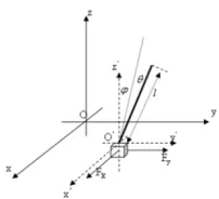
The x- y inverted pendulum which is driven by two horizontal control forces on a pivot is shown in Fig.1, the control action is based on the x-y horizontal displacements of pivot.

According to total kinetic energy and potential energy of the x-y inverted pendulum, the Lagrange’s equations of the x-y inverted pendulum can be deduced as

(1)

Where -0.5x0.5 and -0.5y0.5.According to Eq.(1) ,the state equations of

the x-y inverted pendulum can be expressed as followed

(2) Where                               0 ) ( ) ( ) ( 0 1 0 0 0 0 ) ( ) ( ) ( 0 0 0 1 0 2 2 2 2 2 2 2 y Mml m M I m M mgl Mml m M I mlb Mml m M I gl m Mml m M I b ml I A Ax CONTROL METHODS PID Control

In this paper, the PID control approach is used to track the trajectory which is set by the software and to control the cart at the desired position , PID controller: Angle PID controller or cart PID controller have been designed. The equation of the PID control is given as

dt t de K dt t e K t e K u dp ip pp p ) ( ) ( ) ( 



Where e(t)_{are angle error or cart position error. Since the pendulum angle}

dynamics is coupled to the cart position dynamics, the change in any controller parameters affects both the pendulum angle and cart position, which makes the control tuning of the inverted pendulum tedious. it is the best way to get the optimal the controller parameters by using trial and error methods and observing the responses of Simulink model.

Optimal Control Using LQR

Linear quadratic regulator(LQR) is that whose object is a linear system in the state space form of modern control theory. LQR theory is one of the earliest and

most mature state space design methods in modern control theory. Especially it is valuable that LQR can get the optimal control law of linear state feedback, and is easy to form a closed-loop optimal control.

SIMULATION AND RESULTS

The Matlab-Simulink models for the simulation of modeling ,analysis, and control of nonlinear inverted pendulum cart dynamical system without and with disturbance input are developed. The typical parameters of inverted pendulum-cart system setup are selected as mass of the cart (M): 1 kg; mass of the pendulum (m):0.1 kg; length of the pendulum (l): 0.3m; length of the cart track (L): ± 0.5m; the friction coefficient of the cart and pole rotation is assumed negligible. The disturbance input parameters taken in the simulation are[3]: band limited white noise power = 0.001, sampling time = 0.01, seed = 23341.After linearization, the system matrices used to design LQR are computed as

             0 4 . 29 0 0 1 0 0 0 0 0 0 0 0 0 1 0 A              3 0 1 0 B        0 1 0 0 0 0 0 1 C _       0 0 D

The LQR gain vector is obtained as

1 1.785 25.442 4.6849



K

Here, three tracking control methods have been implemented for the optimal control of nonlinear inverted pendulum-cart dynamical system:

1) PID control method having one PID: this is the cart PID; 2) Two PID controllers method: the angle PID and cart PID 3) LQR control method

In this paper, infinite shape trajectory is proposed, which based on the circular path and is changed the frequency relationship between X, Y direction, The speed of the cart in two orthogonal directions can be set different speed, which increase the difficulty of control. Infinite shape locus function of base is:

The formula can form the movement of "infinite" shape, whose starting point is (0,0) and whose center is (0.08,0) in the XY plane. The base have different speed in X,Y direction, which can make coupling of X-Y inverted pendulum more serious to achieve the base car trajectory tracking control.

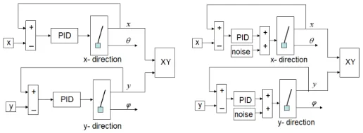
The Simulink models for control of nonlinear inverted pendulum system using cart PID control method for both cases of with disturbance input are shown in Fig 2. The left of Fig. 2. is the block diagram of one PID controller of the x-y inverted pendulum without noise input. The right of Fig 2. is the block diagram of on PID controller of the x-y inverted pendulum with noise input. In two block diagram, the x location and y location in the tracking trajectory are collected into the XY graph.

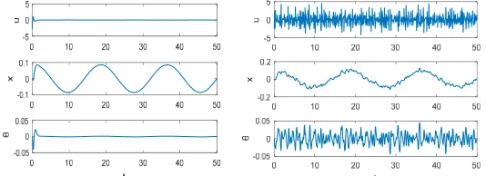
The band limited white noise is added as the disturbance input to the system. The measurement are considered as followed: pendulum angle  _{, cart position x}

and the value of control u. The simulation results are shown in Fig. 3. The left of Fig. 3. is the result of one PID controller of the x-y inverted pendulum without noise input, and the right of Fig. 3. is the result of one PID controller of the x-y inverted pendulum with noise input. From the Fig. 3. the conclusion is that it is easy to control the value of the inverted to the tracking balance under the situation without noise input. But it is impossible that making the inverted pendulum track balance with noise input.

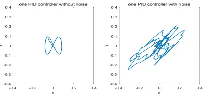
The tracking trajectory of one PID controller is shown in Fig. 4. The left of Fig. 4. is the tracking trajectory of one PID controller of the x-y inverted pendulum without noise input, this result convince that the parameter of PID is suited for this system. The right of Fig. 4. is the tracking trajectory of one PID controller of the x-y inverted pendulum with noise input, from this result, the conclusion can be got that one PID is difficult to achieve the tracking trajectory.

Figure 3. Responses of pendulum angle θ, cart position x, and control force u of nonlinear inverted pendulum without noise(left) and with noise(right).

Figure 4. The tracking trajectory of one pendulum controller control: without noise(left) and with noise(right).

The Simulink models for the optimal control of the nonlinear inverted pendulum-cart system using two PID controllers(angle PID and cart PID) is showed in the Fig. 5. The left of Fig. 5. is the block diagram of two PID controllers of the x-y inverted pendulum without noise input. The right of Fig. 5. is the block diagram of two PID controllers of the x-y inverted pendulum with noise input. In two block diagram, the x location and y location in the tracking trajectory are conveyed into XY graph.

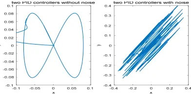
The tracking trajectory of two controllers is shown in Fig. 6. The left of Fig. 6. is the respond of two PID controller of the x-y inverted pendulum without noise input, and the right of Fig. 6. is the respond of two PID controller of the x-y inverted pendulum with noise input. Form the respond of u, x and  , we can get the conclusion that the system is very fast to get the tracking balance without noise input and it can testify that the parameter of two PID controller can control the tracking trajectory. On the contrary, the conclusion shows that it is impossible to achieve the balance of tracking using the same parameter with noise input.

one PID is more difficult to achieve the tracking trajectory than the one PID controller.

Figure 5. Two PID controller of inverted pendulum system: without noise(left) and with noise(right).

Figure 6. Responses of using two PID controllers with noise: without noise(left) and with noise(right).

The Simulink models for the optimal control of the nonlinear inverted pendulum-cart system using LQR control method for both cases of without and with disturbance input are shown in Fig. 8., The left of Fig. 8. is the block diagram of LQR controllers of the x-y inverted pendulum without noise input. The right of Fig. 8. is the block diagram of LQR controllers of the x-y inverted pendulum with noise input. In two block diagram, the x location and y location in the tracking trajectory are showed in XY graph.

The tracking control result of two controllers is shown in Fig. 9. The left of Fig. 9. is the respond of LQR controller of the x-y inverted pendulum without noise input, and the right of Fig. 9. is the respond of LQR controller of the x-y inverted pendulum with noise input. Form the respond of u, x and  , we can get the conclusion that the system is very fast to get the tracking balance without noise input and it can testify that the parameter of LQR controller can control the tracking trajectory. On the contrary, the conclusion shows that it is possible to achieve the balance of tracking using the same parameter with noise input from the respond of cart location x, whose wave form is similar with the respond without noise

Figure 8. The LQR control of inverted pendulum system.

Figure 9. Responses of using LQR without noise and with noise.

Figure 10. Trajectory of using LQR control (left) without (right)with noise.

CONCLUSIONS

PID control and LQR are optimal control techniques to make the optimal control decisions which are implemented to control the nonlinear inverted pendulum-cart system without continuous disturbance input in using tracking control. But in tracking control with noise, the method using the LQR is superior to the methods of PID controller. On the other hand, the anti-interference ability of LQR control is better than that of PID controller. Meanwhile. the design of LQR is very easy than PID.

REFERENCES

1. D. Cheng, Controllability of switched bilinear systems, IEEE Trans. on Automatic Control, 50(4): 511–515, 2005.

2. H. Poor, An Introduction to Signal Detection and Estimation. New York: Springer-Verlag,

1985, chapter 4.287–295.

3. P. Mason, M. Broucke, B. Piccoli, Time optimal swing-up of the planar pendulum, IEEE Transactions on Automatic Control 53 (8) (2008) 1876–1886.

4. C.W. Tao, J.S. Taur, T.W. Hsieh, C.L. Tsai, Design of a fuzzy controller with fuzzy swing-up and parallel distributed pole assignment schemes for an inverted pendulum and cart system, IEEE Transactions on Control Systems Technology 16 (6) (2008) 1277–1288.

5. R. Shahnazi, T.M.R. Akbarzadeh, PI adaptive fuzzy control with large and fast disturbance rejection for a class of uncertain nonlinear systems, IEEE Transactions on Fuzzy Systems 16 (1) (2008) 187–197.

6. A.M. Bloch, N.E. Leonard, J.E. Marsden, Controlled lagrangians and the stabilization of mechanical systems I: the first matching theorem, IEEE Transactions on Automatic Control 45 (12) (2000) 2253–2270.