I Nonlinear gas oscillations in pipes II Wavetrains with small dissipation

II. WAVETRAINS WITH SMALL DISSIPATION.

Thesis by Javier Jimenez.

In Partial Fulfillment of the Requirements

for the Degree of Doctor of Philosophy

California Institute of Technology Pasadena, California

1973

ACKNOW LEDGEMENTS.

It is a pleasure to acknowledge ITly gratitude to all those who made possible my graduate study and the writing of this thesis.

The work on part I was motivated by the experiments on non-linear resonance conducted by Professor B. Sturtevant. I am indebted to him for ITlany helpful discussions.

I wish to express ITly appreciation to ITly advisor Professor G. B. Whitham for his guidance and direction of the present

work, specially in the second part.

The advice of Professor H. B. Keller was helpful in the nUITlerical solution of the p:cobleITls in part 1. Also Professor H. W. Liepmann offered some very needed guidance during the first part of my stay in the Institute.

I am specially grateful to Ms. Anna Castro for her help in typing the manuscript.

ABSTRACT.

In part I of this thesis we study theoretically the problem of forced acoustic os ciIlations in a pipe. The oscillations are produced by a moving piston in one end of the pipe, while a variety of boundary conditions ranging irom a completely closed end to a cOITlpletely open I.TIouth are considered at the other end. All these boundary conditions are modelled by two parameters: a length correction and a reflection coefficient equivalent to the acoustic impedance.

Tbe linear theory predicts large amplitudes near reso-nance and non-linear effects becolTle crucially irnportam:. By expand-ing the equations of alotion in a series of the Mach num.ber, both the amplitude and wavefoTlTl of the oscillations are predicted there.

In both the open and closed-end cases the need for shock waves in SOITle range of parameters is found. The aITlplitude of the oscillation is different for the two cases, however, being proportional to the square root of the piston amplitude in the closed end case, and to the cube Toot in the open end.

This part of the thesis was first published in the Journal of Fluid Mechanics.

Lagrangian depends on the variable and the solution of the prob-lem 9 and which can be used to describe irreversible proces se s.

TABLE OF CONTENT.

PART

PAGE

L Nonlinear gas oscillations in pipes.

1. Introduction. 1

2.

General equations. 7

3. Perturbation scheme.

3. I Basic expansions. 12

3.2 Closeci end case 18

3. 3 Open end case

19

i. Analysis of the closed end case 23 Results fOT the open end case 34

6.

Conclusions. 41

References. 43

Figures. 45

II. Wavetrains with small dis sipation.

L Introduction. 55

? _{~. Variational principles for irreversible systerfls.}

2.]. Reversible and conservative systems.

2.2: The beauty of conservation laws. 0+ 2. 3 Variational principles for irreversible

systems.

67

3. The averaged Lagrangian technique.

PART

3. 2 Irreversible systems. 4. The gene ral method.

4. 1 The zeroth order approximation. 4.2 Formal justification of results. 4. 3 Partial differential equations.

References. Appendix.

PAGE

79

86

90

97

1. NONLINEAR GAS OSCILLATIONS IN PIPES.

1. Introduction.

The problem we consider is the oscillation of a gas inside a pipe of length Ljl and whose transverse dimension is small with respect to the length. At one end of the pipe (x

=

0) a piston executes small harmonic oscillations with a frequency that we choose to be of the order of the resonant frequency associated with L. At the other end (x

=

L) we want to model a range of physical conditions progressing from a completely closed to a completely open tube, including different kinds of perforated end plates or other mouth configurations, thereby producing varying arnounts of coupling to the room.

The imaginary part corresponds simply to a length correc-tion. The effective length of the pipe is different from the rea] length. and this difference accounts for part of the

two-dimen-sional effects at the mouth section. There are some classical theoretical results (Rayleigh 1945) aiming to predict the value of this correction, based on assumptions like potential flow near the pipe end, and no viscous effects. In the real world, however, these assumptions are hardly ever fulfilled except for the small-est amplitudes of the gas oscillations. In any case, as the cor-rection arises from transverse effects, the general order of magnitude can be expected to be no more than a few pipe diam-eters, and this should cause no qualitative difference in the behav-iour of a slender pipe.

In a similar way. the real part of the impedance can be interpreted as a partial reflection coefficient. The general idea is that, from some diameters away, the pipe end should look like a virtual plane section. A long wave running into this section from the pipe is partially reflected and partially transmitted, or

In summary, although the impedance model was created

for linear oscillations, it still provides a very compact way of treating a wide range of physical cases. In fact, there have bc(~n

several attempts to justify its use in the treatment of acoustically absorbant materials at high radiation intensities where nonlinear effects appear. Thus, in 1967, Ingard and Ising. using experi-ments with resonators, proved that the behaviour of orifices could be successfully approximated at moderated intensities by the use of an amplitude-dependent impedance coefficient.

The experiments undertaken to complement the present work (Sturtevant 1973) have been carried out at much higher intensities than in previous cases. Therefore it is of interest to check them against the predictions of the impedance m.odel and, in that way, to judge the validity of the model itself.

Here we, therefore, develop a nonlinear theory applicable to those cases in which resonance peaks occur with sufficient amplitude that linear analysis is inadequate. The first suggestion of the importance of nonlinear effects was rnade by Lettau (1939) who observed experimentally the appearance of traveling shock waves near the linear resonance frequency in both closed and open tubes.

of the solution, he was able to prove that the nonlinearity of the equations alone bounds the resonant amplitude away from infinity without recourse to dissipation, as well as to compute waveforms in qualitative agreeITlent with the experimental results.

Saenger and Hudson (1960) further refined the experimental observations and atteITlpted to account theoretically for the effects of viscous shear and heat conduction. Finally, Chester (1964)

developed a consistent theory for the closed pipe in which, with-out any special assumption, the appearance and strength of shock waves, as well as the detailed waveforms for all frequencies, were predicted. One important result of his paper was to show

1

that the amplitude of the pressure oscillation is O(02j whereas the piston amplitude is alUch smalle:c, 0(6). Temkin (1968) ob-tained still rrwre experim.ental data on the closed tube and gave a simple but elegant account of the different effects present in the probleIYl using energy balance considerations.

Wijngaarden (1968) treated the case of an open pipe at resonance using a nonlinear boundary condition in which viscous dissipation caused by flow separation at the pipe exit was as-surned to dominate radiation losses and. in fact, the nonlinear behaviour of the gas in the pipe itself. This is probably true for some range of the geometrical parameters of the pipe and represents the opposite extreme to the case treated in the

pres-1

but this is governed primarily by the dissipation boundary con-dition.

Mortell (1971) attempted a straightforward generalization of Chester' s analysis of the closed pipe to other cases of non-linear oscillations, including the open pipe with a perfectly reflecting exit. It turns out, however, that the method does not generalize to this case without special precautions, and Mortell derived the wrong result. In particular, the amplitude of the

1

oscillation was mistakenly given as 0(62).

The first author to point to the correct result was Collins (1971). who studied the problem of a nonlinear wave equation applied to the vibration of a string. He correctly expanded the equation in terms of the resulting amplitude, instead of the forcing amplitude, pointed out the similarity to the open pipe,

1,.

and predicted the resulting amplitude to be 0(03 ). He did not

present detailed calculations for the gas dynamics case. and. in particular, failed to point out the presence of shock waves in the solution.

A closely related class of problems was treated by Chu and Ying (1963), when they studied thermally induced oscillations in closed pipes. They used a characteristics perturbation proce-dure due to Lin (1954) which is very close to the one used in this work.

2. General equations.

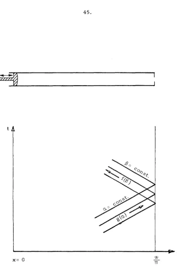
Consider the pipe along the x axis. The passive end of the pipe is located at x= L. At x= 0 a piston oscillates according to the law

,...

x

=

-1. cos wt

and this causes the gas to vibrate around an equilibriuITl state given by a sound speed a and zero gas velocity. By making

o

velocity and tiITle non-diITlensional with a and TT

/'US

respectively, o

we have the sound speed fluctuating about the value 1 and the period of the oscillation fixed for all driving frequencies and equal to

2.

When we change the driving frequency, however, the uni t of length change s and the pipe ha s a va ria ble length in the new coordinates, with the passive end located at

where

,...,

wL

x = -TTa

o

...

WL

W=

-a o

ill TT

is a non-diITlensional measure of the forcing frequency.

(2. 1)

(2.2)

The motion of the piston, however, has a constant frequency, and is given by

x=

[)

-- cos TTt .

The parameter 6

6

=

wi, _a o

i,

-w-

_L (2.4)

is now a good indicator of the strength of the forcing terms. and is in fact a Mach number for the motion of the piston and for the motion of the gas near the piston.

One might assurne then that 0 also measures the strength of the gas oscillation everywhere in the pipe, so that, if 0 is small the linearized acoustic equations would be applicable.

If one tries to do that, one gets consistent results for all values of

w

except for those pipe lengths which are near reso-nance with the piston frequency. At these values of

w

the motion

of the gas is much larger, in general, than 6 and it becomes necessary to include higher order nonlinear terms in the equa-tions of motion. It should be noted, therefore, that the correct expansion parameter should be the typical Mach number of the gas, which we take to be <::. not the velocity pararrleter of the piston 0, and that one of the aime. of the theory should be to find the relation between 6 and €.

We first write the general equations of rnotion, consid-eTing the gas to be ideal and isentropic, and the motion to be one-dimensional. The velocity of the gas is u and the sound

(Cou-rant & Friedrichs 1948)

On

~~

= (u-a-l)

~~

ax

(it

as

=

(u+a+1)as

2a

2£(13 )

- - -u = y -1

2a

2g(0.) Y-1

+u

=

,

a.

=

13 ,

x = 0 and t =0..

On x = TI cos TIt, u

o

= g(o.)-f(l3) = 0 sin TIt.

(2. Sa)

(2. Sb)

(2.

6a)

(2. 6b)

(2.7)

(2. 8)

Equations (2.5) define the geoITletrical coordinates, x and t, in the characteristic plane, and (2.7) ITlakes the definition unique by choosing

a.

and

13

to be the tiITle t at x = O. In the pipe

a.

is constant along the C+ characteristics and

13

along the C charac-teristics. Equations (2.6) define the invariants riding each faITlily of characteristics. In particular g(o.) can be considered as a

"'simple" wave going to the right, and

£(13)

as the left-going reflected wave. Equation (2.8) is the boundary condition at the piston.

The only remaining equation is the boundary condition at the pas sive end of the pipe, and, following the discussion in the introduction, we assume it to be:

where b is a number between

+

1 and -1, which gives the frac-tion of the right-going wave that is reflected back into the tube. The condition that b be bounded between

+

1 and -1 obviously means that no energy is created at the passive end, or, more specifically. that any radiated energy is transmitted from the pipe to the room, and not vice versa. It is easily seen that the value b = 1 corresponds to zero velocity at the end section and is equivalent to a perfectly closed pipe, while b

=

-1 implies a

=

0 and represents an ideally open end, at which the pressure is always equal to room pressure.

Equations (2.5) to (2.9), plus the periodicity condition which says that we are looking for a steady oscillation of the sam.e period as the piston, completely define the problem.

If we assume now that u and a are 0(0) and O~ I, we can neglect the second order terms on (2. 5) and apply the piston condition at x

= o.

The result is the classical linear theory. The characteristics are parallel straight lines and the solution for f(!3) is sinusoidal with amplitude

(2.10) When b is close to ± 1 this aITlplitude has sharp resonance peaks in

w.

There the oscillation is rn.uch larger than 0(0), and the nonlinear effects m.ay be expected to be important. For b fa r from these values, however, the linear theory is correct for

remain of order

o.

A particularly interesting case arises for b=O, when the amplitude of the oscillation is completely independent of frequency. This is, of course, because no wave is reflected from the pipe end and the oscillation is just the simple wave produced by the piston, travelling undisturbed to infinity.

Therefore, the only regions in the b-w plane where linear theory should not be expected to hold are very small regions whose extent logically depends on the size of E:. Their location

can be derived f:com the linear theory and falls into two families. Almost-closed pipes, where b is near +1, have resonance peaks

at w~n,2n,3n, . . . , and almost-open pipes, with b near -1,

n 3n Sn resonate at w~2 '

Z- '

-2- •...

An asymptotic theory tTying to explore these regions for small E: should include, then, expansions for band w as well as

3. Perturbation scheme. 3. 1 Basic expansions.

The first question to be solved is the relation between

€, the Mach number of the gas, and fl, the piston motion. We

have seen that assuming both to be of the same order leads to a first order solution for the velocity that is inadequate near resonance. This suggests that the nonlinear behaviour of the wave should be made to balance the forcing term, and as this nonlinearity can be expressed as a power series in €, it is logical to expect that fl can be equated to SOITle integer power of €:

(3. I)

The value of N has to be assumed at the beginning of the pertur-bation procedure, and the test of the a~sumption is the consis-tency of the resulting analysis. If the as sumed value of N is too low, we will get essentially the linear theory (N=l), and if too large the solution will be identically zero to the first order, contrary to the assurrlption that € is the order of the oscillation.

the cor rect perturbation procedure is by Poincare's method. The use of characteristic coordinates here corresponds to the expansion of the independent variables used in that case.

If a. and [:3 are, then, considered as the independent

variables, the appropiate expansions for u and a are

a u

f( [:3 )

z

Y-l -

"2

=

= 8f1([:3)

+

8 fZ(~)

+

(3. Z) a u

g( a.) € g 1 (a.)

+

€ 2 g2(a.)

+

Y-l +"2

=

=

The geom.etrical coordinates x and t must be expanded too in powers of €. We take

2

x=xo(0..,~)+8xl+8 x_Z+···

2

t

=

to (a., ~)

+

HI

+

E: t

z

+ ...

(3. 3)

Using these expansions in the equations for the characteristics (2. 5) and separating orders, we get for all n

n ()

-~

{

Y+l y-3

} -2-

t "a. (x +t ) - -2- f. (~)+ -2- g. (a.)

d n n 1 1 80.. n-i

1=1

n (3.4)

a

L

{

Y

i

3 £i(!3)+ Y;l gi(U)

}

..2...t - (x -t ) =

8[:3 n n

i=l 813 n-i

The corresponding boundary conditions (2.7) are expanded to:

At a. = [:3 ; x = 0 and t = a. ,

o 0

x = t = O ; n:2:1.

n n

The system of (3.4)-(3.5) can be solved recursively in terms of the f's and g's. The first two orders in x and tare

x =1-(I3-a), t =1-(13+0.),

o 0 (3. 6)

which correspond to the linear characteristics, and

where

xl = Y;l (l3-a)[ f

l (I3)+gl(a)] +Y

S

3

['l'l(I3)+~l(I3)-'l'l(o.)-~l(o.)]

(3. 7) tl = Y;l (\3-0.)[ f₁(\3)-gl(o.)]

+

Y;3

['l'I(I3)-~I(\3)-'l'I(o.)+~I(o.)]

,

a.

'1'. (a)

1

=

J

gi(S)dS

a.

(3. 8)

~.(o.)

1

=J

£.(S)dS 1

Similarly, x

2 and t2 can be computed as functions of f1, g I' f2 and g2' and xn and tn as functions of the f

i, gi up to n only. This fact makes for an ordered expansion procedure in which higher order terms do not "feedback" to lower orders.

It should be noted that the system (3.4)-(3.5) together with the definitions of f. and g. in (3.2) contain all the equations

1 1

of motion of the gas, and,. in particular.,. all the nonlinearities of the probleITl. All that remains now is to apply the boundary conditions to find f and g.

The first boundary condition is the one at the piston (2. 8).

g.(a) = f.(a) ; i< N

1 1

(3.9)

This condition halves the nUITlber of unknown functions by elimi-nating the g .. Physically, the wave in the pipe does not "see"

1

the piston up to order N, and if N

>

I, the solution is essentially a free standing wave, with its shape deterrr"lined by the piston only through the higher order terms. As N

=

1 corresponds to the clas sical linear theory, near resonance we must actually have the situation N> 1.

Next it is necessary to introduce the condition (2.9) at the pas sive end; this condition includes the parameters wand b.

From the discussion in the last section we know that these param-eters should be expanded around their values at resonance,

(3. 10) I _{.J ,}

where the two first resonance peaks correspond

to

Open end: b = -1 w = TT

/2

,

0 0 _(3.11)

Closed end: b =

+1

w = TT

0 0

The position x

=

ill

ITT

of the passive end will now be mapped into a certain line in the

a.-t3

plane

To compute it expand

(3.13) Then substitute (3.12) in the right hand side of (3.13), expand the x.(~,a.) in Taylor series, and equate like orders to solve

1

,...., for

13:

2w

j3 (a.)

=

0.+

_ 0

o TT

(3.14)

Equations (3.14) can be expressed in terms of the f .. Once

1

again, the solution is ordered in the sense that

f3

(a.) does not

n

contain terms from orders higher than n. Finally, we use all these expansions in the reflection condition (2.9), which can now be written as:

Expanding the right hand side in Taylor series and separating orders:

0(8 ): (3. 1 Sa)

f

2(a.) -bof2(So)

=blfl(a.)+boSl(a.)f~(So)-ON2sinTTa..

(3.15b)

where 0NM denotes the Kronecker delta.

This hierarchy by itself does not allow the calculation of the f., unless we impose some conditions on the solution,

1

which, in fact, correspond to the initial conditions neces sary in the hyperbolic problem. As we are looking for steady

oscillations. we impose the condition that the solution must be periodic with the same period as the piston. But, since a. and

~ correspond to real time at x = 0, periodici ty in time means directly periodi city in a. and ~. So, the desired condition is that the f. (a.) be periodic with period 2, i. e.

1

£.(0.) =£.(a.+2} for all l .

1 1 (3.16)

3.2 Closed-end case.

Doing first the closed end case, we start by assuming that N = 2 (N = 1 would give the classical linear theory). From (3.11) and (3.14), ~ =0.+2, and the left hand sides of (3.15)

o a re of the type

£.(0.) -£.(0.+2) ,

1 1

and, because of periodicity, they are all identically zero. The desired set of equations is then given by the right hand sides of (3.15) equated to zero.

The equation for 0(8), (3. 15a), is satisfied identically and gives no information, but the second equation 0(82), gives an equation for i1

(3. 17)

with

2

<f1>=iJOf1(S)dS (3.18) representing the rnean value of f1 over one period. For b

3. 3 Open end case.

For an open end b ::: -1 and 13 ::: 0.+ 1, so that the left hand

o 0

sides of (3.15) are of the type";

£.(0.) +£.(0.+1)

1 1 (3.19)

and do not vanish in general. However, if the f. have period 2,

1

the expressions in (3.19) have period 1, and that imposes restric-tions on the right hand sides, which give the desired equarestric-tions.

In pa rticula r.

[ R. H. S. ] . (a) ::: [R. H. S. ] . (0.+ 1)

1 1

(3. 20)

is an equation involving only the f up to order i-I. FraIn the first order in (3.15) we get

(3.21)

so that the waveform changes sign as we advance a semiperiod. This is important because it means that any shock wave in the so-lution implies an expansion shock half a period away. It should be :remembered that the original equations were isentropic, so

expan-.

sian discontinuities are not really inconsistent in lower order ap-proximations. On the other hand. we will see later that fl cannot be calculated until we include third order effects, so that the isen-tropic assumption breaks down with the presence of shocks of O( E:). We will come back later to this problem.

the corresponding equation (3. 20) we get, after some algebra, i

b 1 f 1

+w

1 f 1

=

s in TT

a. •

(3.22) which is linear and has no bounded solution for the case

b

l =WI =0. corresponding to resonance. That means that the as-sumption N=2 was wrong and that we should go to higher order. For N > 2, (3.22) appears with right hand side zero. Therefore, b

I and

wI

have to vanish in the resonance band, as the homoge-neous part of (3.22) has no non-trivial periodic solution.

The physical interpretation of this result is that the res-0nance band in this case is, at most, 0«(';2) and the piston motion O(e: 3). Outside this region we recover again the linear theory.

As suming then

(3.23)

and repeating the proces s for (3. 15) up to third order. we get, after a great deal of algebra, an equation for fl

(3.24)

where

(3.25) 2

period is zero because of (3. 21).

The correction to the frequency given by (3. 24) in the open-end case is then of the same type as the one given in (3. 17)

for the closed end, and both can be interpreted as a shift in the linear resonant frequency due to the difference between the real mean pres sure and the pres sure defined a priori as mean.

It is interesting, in fact, to examine the validity of the separation of the pressure (sound speed) waveform into a mean value and a perturbation, particularly as this separation is usual-ly not clearcut in nonlinear problems. In this case, however, a

clear definition of a=O is introduced by the boundary condition at x=L, as this condition is linear. In fact the reflection condition is equivalent to making a ... u. except for b exactly equal to 1. With that exception, then, a=O corresponds to the state at the pi-pe exit when u=O, and that can, in principle, be related to am-bient conditions.

The special case b=l corresponds to the completely closed pipe and the gas in the tube, having no connection with the

atmo-sphere,does not have any clearly defined reference pressure. This is reflected in the equation (3. 17) where <£1> can be deter-rn.ined for all cases except b

i =0. Integrating (3. 17) over one

period. we get

2

w

<

f'

> - (y

+

1 ) < f

i

>

+

b < f

>

=

< sin TT

a.

> .

1 I I I 1 1

of periodicity as does the right hand side, so we get b

1 <f1 > =0. If b

1

f:.

0, fl has to have zero mean. If b1 =0. <f1> is not fixed and we know from the previous discussion that we can define it

arbitrarily. To preserve continuity of the solution with b 1 we define a5

<fl> =0 (3.26)

for all b

4. Analysis of the closed-end case.

We now corne to the problem of actually solving the equa-tions (3. 17) and (3.24) to find the response of the system near the two resonances. The first difficulty is that both equations are singular for some values of the parameters, and the effect of these singularities must be studied before we attempt a

numer-ical treatment of the equations.

Consider first (3.17), representing the closed ended case. Following the discussion at the end of the last section, it can be simplified to

with the boundary conditions f

l(0.+2)=fl(0.) •

<f1

>=

iS~fI(S)dS

=

°

(4. 1)

(4. 2)

(4. 3)

For all b

l

f

0, (4.3) is redundant and follows directly from peri-odicity. In numerical calculations, moreover, (4.2) proves to be much easier to use. as it reduces the order of the problem by one. When b

l =0, however, (4.2) is automatically satisfied and (4.3) must be used. In this case, though, the equation can be integrated exactly, and there is no need for nume rical work.

It may be well at this point to remember the significance of the parameters b

W~ TT ( 1+ E:W I) ,

(4.4)

b~ 1-E: b

I

and note that W I represents the distance in frequency from exact

resonance, and b

I indicates the deviation of the end condition from the perfectly reflecting closed end, or, in other words, the amount of wave radiated to the exterior. It follows that negative values of b

I have no physical significance, and that the range of parameters to be studied is the upper-half plane in b l-w 1 space.

The origin of this plane represents the perfectly closed pipe at resonance, and so, as we move away from it, we should approach the results of the linear theory. In fact, if in (4. 1) we let b

I or WI grow large. the nonlinear term can be neglected and we get asymptotically the linear result

-I

X

=

tan

(4, 5)

Another useful property of the system (4.1)-(4.3) is that it is invariant to the transformation

f ₁ (0.)'- -f (-a.) _{1 · ,}

WI -+ -w 1 ' (4. 6)

....

it to all frequencies by using (4.6). In what follows we always assume that wI is positive.

We now solve (4.1) for the special case b

1=O, and,as

stated before, the solution should reduce to the results given by Chester for the completely closed end. The equation can be inte-grated directly to

y+

I 2 1

2w₁f₁ - - 2 -f1 +TI cosTIa. = const. (4. 7) or

2W 1 2 1. 1.

fl = Y+l - [TT(Y+l)J2 (K+COSTIa.)2 (4. 8)

where K is an integration constant to be determined with the help of (4.3). In attempting to do this, however, we get a transcendental equation in K involving elliptic functions which has a real root only if

(4. 9)

For all other values of wI' then, there is no continuous solution satisfying (4.1) and (4.5). Chester (1964) interprets this fact as an indication of the appearance of shock waves in the flow, and this is confirmed by experiment.

speed of propagation of this discontinuity is just the arithmetic mean of the wave velocities immediately in front of and behind it. This property. and the fact that a shock travelling along one

set of characteristics does not modify waves travelling along the other set, contains the cmnplete shock relations to the order needed.

By using periodicity, the jump conditions across the shock discontinuity can now be determined.

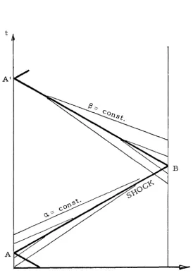
Denote by + and - superscripts the conditions in front and behind the discontinuity and consider first a shock, as AB, travel-ling to the right (see fig. 2). To first order, this shock is

always located at a given value of a.,

or, expressed in terms of f 1,

Therefore, along the shock

say a. , and its speed is s

(4. 11)

V

dx =(1+E:V

l )dt =dt +E: -2 1

d~

s s s (4.12)

Integrating this equation from A to B, and using the known values of x (A) and x (B). we get

s s

Note that, here, we can not use the condition that <fl>

=

0, which was derived using the continuity of the solution. Repeating the

proces s for the left going shock, BA', and combining both re-suIts, we get

(4. 14)

But periodicity imposes that this difference be exactly 2, so the shock relation reduces to:

(4. 15)

This is, however, still not enough to completely determine the solution, as <f

>

is left unknown.

1 We can get this

informa-tion by integrating (3. 17), in much the same way as with the con tinuous case, from just in front of the shock to just behind the shock one period ahead. Then

+

-[w"- _

y+l f 1H

1J [ f- +

1-f1

J

+bl <fl

>

=0 •

1 2 2 (4.16)

and using (4.15) we have

(4.17) for all cases except b

l = 0, where (4. 17) can be fixed by definition as before.

to-gether segments of continuous solutions of (4. 1) with jumps sat-isfying (4. 15). Detailed examples of waveforms constructed in this way are given by Chester (1964) for b

1

=

0 , so we turn our attention to the more general case where b

1 ~ O.

We can expect that in those cases, too, it will be neces-sary to introduce shocks for some range of parameters and, so, we must study first of all the question of existence of continuous solutions;this obviously depends on the behaviour of the singular-ities of (4. 1). We study these singularsingular-ities next.

They occur in the f1 - a. plane, when the coefficient of

I

f1 vanishes, or

2w

f =_1

1 y+ 1 (4. 18)

and the solution f1 (a.) is only affected by them when it has to pas s trough that value. For large values of wI' that can only happen for very large amplitude waves. However, the asymptotic

solution (4.5) suggests that the amplitude really decreases as wI increases, so condition (4.18) is never realized for large

w

₁ and

'-continuous solutions should be expected for that range. Once a continuous solution has been shown to exist, it is easy to convince oneself that it is unique.

and, to do this, we expand the equation for small displacements around (4.18). In particular, let

(4.19)

where cP is some general value of

a.

in the neighborhood of which we want to study the solution. Substituting in (4. 1), we have

(y

+

1) g g! - big = ( Y

~

1 b 1 WI - sin nip) - ( nco snip) x

+ ....

(4.20) There are two pos sible cases, depending on the cP chosen. In most instances the constant on the right hand side of (4.20) is not zero, and the behaviour of the solution is then given by

(4. 21)

The exact shape of g depends on the sign of the constant in brack-ets, but it always includes a branch point at x

=

0, giving two-val-ued solutions which are inadmissible from a physical point of view (see table I).

If, however b W ::; y+ 1 there are two points in every 1 1 2 I

cycle in which the constant term in (4. 19) vanishes. Name these point as

-+

-+

~~~

~

-+-

~~

..

H H H

>-H H H H

... 1'" "'1'"

~

IN_

~

N

-...

...

+ +

'ZI< ... _>- "<t' ...

>-..0 ~

N ..0 N

t= t=

'.D '.D

I ... :

...

I I

...

...

~ ~

... 1 ...

+1..0

.../

...

>-N +..0 >-N

V 1\

.--< r - i

3 3

...

---3 ...

...

-

... + 3 _... ... ..0

>-+ N

..0 _~ ...

N I

""#.. C

I

...

8-I

8- <IJ t=

C II II

...

<IJ +

8- +

8-~IN

>-VI _...

3 _...

-

+

~ =TT - ~ (4. 22b)

The leading ter:ms of (4.20) near those points are

(y+1)gg' -bIg+(TT cosTTi.P)x= 0 . (4.23) This is now a bilinear equation, which can be solved exactly (Birkhoff & Rota 1969). The type of the solution depends on the behaviour of a particular quadratic algebraic equation involving the coefficients of (4. 23). As the value of q, in (4. 23) can be ex-pres sed through (4. 22) III terrns of b

l and wI' the nature of the singular points can be classified in ter:ms of these paraITleters alone.

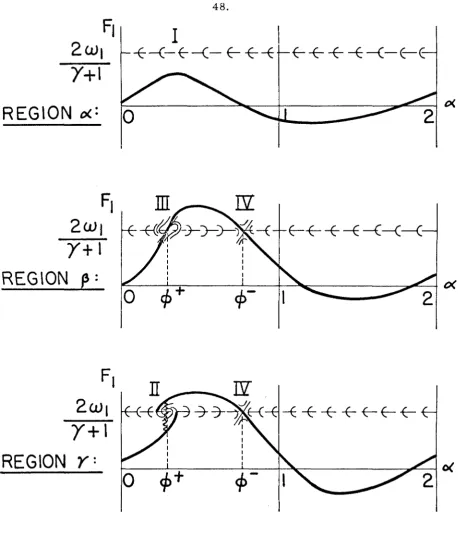
A su:mITlary of the ITlost iITlportant results of this c1as sifi-cation is given in table 1. Fro:m this table it is clear that if a continuous solution is to cross the singular line (4.18) anywhere, it has to do it through one point of type III or IV. In fact, if it

crosses the line at all, it has to cross it twice, once at q,

+

and another at q, • and because of the shape of type III, it has to

eros s at

~

+ going up, and co:me back at q, - going down. If now, :maintaining the sa:me b

I, we start decreasing wI' the point at 4+ starts to flroll-up" fro:m type III to a spiral point of type II. At the ITlo:ment that this happens, and <I> + becoITles of type II, the

so-lution is no longer able to cross the singular line through that point, although it is still able to get back through ip • At this

+

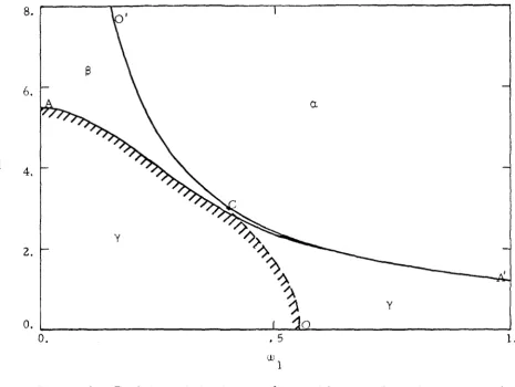
Thus, the nature of the singular points divides the b l -w 1 plane into regions, and in each region the pos sible types of so-lution are different. This classification is presented in figures 3 and 4. These, and all subsequent figures are drawn for air

(y

=

1.

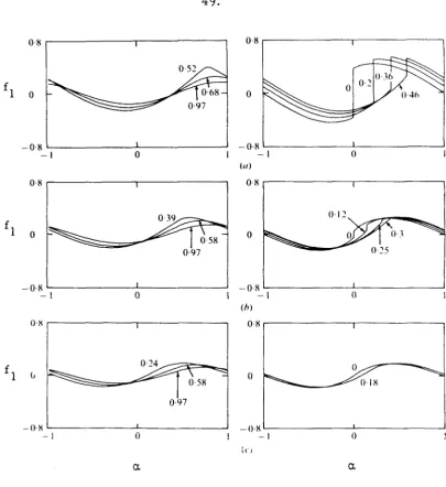
4), although a simple change in scale will adapt them for other values of Y. The waveforms given in figure 4, are those of the pos sible singular solutions in each region. In each case it is pos sible, in principle to have. besides, a continuous solution which never crosses the singular line, like that in region

a..

The

existence of this solution can be best decided by trying to inte-grate the equations numerically to find it.

The process used by us was a second order "shooting" scheme (Keller 1968), starting from large wI for a fixed b

l with the asymptotic solution (4.5) and working inwards keeping b

l co~ stant and decreasing wI ' until the solution touched the singular line. The points in the bI-w

i plane where the solution first touch

ed this line are given by 00' in figure 3. To the right of that line the solution is continuous and nonsingular. To the left, the

solution has to cross the singular line and the best way to find

+

.

it numerically is to start integrating from ~ wlth the slope giv-en by the analysis of the singular points and integrate forward and backwards until the solution crosses the singular line again. A shock can then be fitted, if needed, -using (4.15).

The calculations show that, in the regions

a.

and ~, it is always possible to find a continuous solution for f

derivative may be discontinous at ip- in some cases. The region of the b

l -WI plane where the solutions contains shocks is then only the part OCA of Y lying to the left of 00'.

All this discussion belongs, of course, only to the case of wI> O. For negative wIthe results are completely symmetric,

ac-cording to the transformation (4. 6).

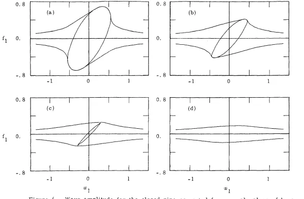
Finally, figure 5 gives some examples of waveforms com-puted for three different values of b

l and several wI' using the method outlined above. Figure 6 is a plot of wave amplitudes as a function of wI for various values of b

l . The four quantities repre-sented in each plot are respectively the maximum and minimum values of f

1, and the values at the top and foot of the shock. It is to be noted that, although a shock is present in the solution for relatively large values of b

5. Results for the open end case.

We now turn our attention to the pipe with the open end. The pertinent equation is (3.24)

sin TTa.

(5. 1)

and is to be integrated in the interval (0,1) subject to the condi-tion

(5. 2)

The results can be extended to the full period (0,2) by using

fl (0.+1)

=

-f

1 (a.) (5. 3)

The significance of the parameters b

Z and W

z

is similar to the corresponding ones in the previous section, and, here too, b

2 is essentially a non-negative number.

The whole problem is mathematically very similar to the closed end case, and most of the analysis carries through

direct-ly to (5. 1). The singularities in this case are located at

so they form two singular lines, instead of one. From (5.4), too, these lines are only real when

w

continuous and well behaved; this is of course also true for

w

2 sufficiently negative.

For intermediate values of the frequency, however, the solution eros ses the singular lines and exhibits the same kind of phenomena as the closed end solution. The analysis of the singular points runs exactly parallel to the one there, and, in fact, the approximate equation near (5.4) is also bilinear in this

case, the only difference being that the roles of the points ip+

and ip are interchanged. The fact that there are two singular lines instead of one does not affect the results much, because it turns out that each line interacts with only one half period of the waveform, as could be suspected from (5.3). In particular, the interval (0,1) is only involved with the plus sign in (5.4).

There are, however, several important differences between this and the closed end case. The first one is the existance of a shift between the effective frequency

w

2' and the physical quantity

w

Z. This shift vanished in the closed pipe, as we were able to show that <f1 _... > was always zero. In (5.1), however, the shift

de-pends on

<f~

>

which is a strictly positive number.

The significance of this shift was dis cus sed in section 3. and its effect in the system is to tilt the resonance peak toward lower frequencies, this effect being more pronounced as b₂

be-comes smaller and the wave amplitudes grow larger.

W

2 as a paraITleter, and after the solution is found, w2 is COITl-puted using (5. 1). The results presented in this section are for Y=l. 4, but, due to (5.1), the change to other gases no longer corresponds to a siITlple change in scale.

The division of the b

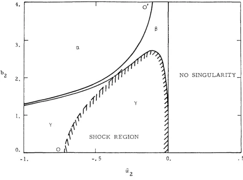
2

-W

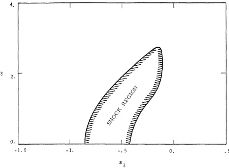
2 plane according to the type of singularities is plotted in figure 7. where the naITle of the regions correspond roughly to the descriptions given in section 4. The solution pas ses through the singular lines in the region between the 00' line and the b

2 axis. The only region qualitatively dif-ferent froITl the closed case is the one to the right of the ordinate axis, where no singularities exit and the solution is always contjn-uous. The shock region is given by the .area of region y to the right of 00' and, in figure 8, it is plotted in "physical" b

2 -w2 coordinates.

A very iITlportant difference with section 4 occurs, however, in the behaviour of the solution within the shock region. The

main reason for it lies in equation (5.3), for this equation as-sures that anything that happens in one seITliperiod. will happen with

opposite sign half a period later. In particular. any cOITlpresion shock in the wave must be followed by an expansion shock of the saITle strength, which is physically quite unlikely.

Even ITlore iITlportant is the fact that (5. 1) really derives 3

of O(e:) first appears in the equations at O(e: 3), so that the assumption of isentropic flow is inconsistent with the existence

of shocks. This is reflected mathematically in the impossibility of finding any condition for a discontinuity in the solu-tion to represent a shock, equivalent to (4.15) for the closed case. In fact, as we try to repeat the process in section 4. to get this kind of condition, we run into the difficulty that any effect produced by the shock is cancelled by the opposite expan-sion shock somewhere during the period.

The influence of entropy production on the solution has another effect on the attempt to formulate a physical model includ-ing this influence. The flow in the pipe is supposed to be peri-odic, so that the entropy produced by one passage of the shock at one point has to be removed somehow before the next passage. The way this entropy is removed is, of course, by cooling the fluid through the walls of the tube, and the modelling of this cooling depends on the exact experimental set up, and introduces new parameters in the problem.

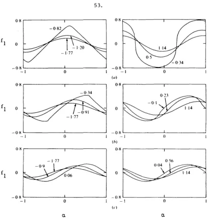
Some representative waveforms computed for three differ-ent values of b

2 and several frequencies are given in figure

9.

For the first two values of b

2 the solution cuts across the shock region so that only results for the frequencies on either side of the boundary are shown; in those cases, the tendency for shocks to form can already be seen quite clearly. The third value of b

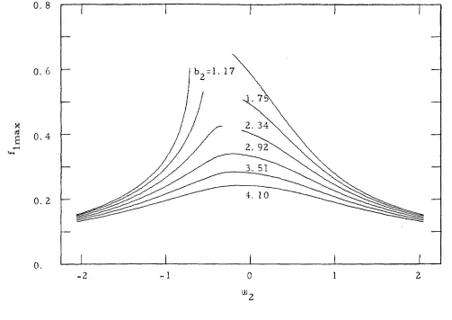
2 is above the shock boundary and so the waveforms can be com-puted for all frequencies and is always continuous. In figure 10, the half amplitude of the wave is plotted versus frequency with b

2 as a parameter. The gaps in the curves correspond to regions with

shocks.

The most important result in connection with the open end case is, however, connected with orders of magnitude. Going back to the definition of O. as measuring the amplitude of the piston motion and E: as measuring the strength of the gas motion, we see that in the closed end E: =0

i,

while in the open end 8

=

0

~,

and the oscillation is in fact stronger when the end is open.

with itself, acts continually and becom.es eventually im.portant. This nonlinear effect appears in the equation at 0(82) and helps "kill" the linear resonance.

For an open end the sign of the wave in the pipe changes eve ry tim.e it is reflected at the open section, and so any pa

rtic-ular signal is a com.pression half of the tim.e and an expansion the other half. So, the steepening by interaction of the wave with itself never accum.ulates, and it is only after third-order interactions com.e into play that the linear resonance can be lim.ited.

It is im.portant to realize on the other hand that, from. the point of view of the energy, an ideal open end is as closed as a rigid wall. In fact the energy flow out of the end section is given by

E=§pdV (5.5)

where V is the volum.e of the gas originally in the tube. For the closed pipe dV=O at all tim.e and the energy flow vanishes. But for the open pipe the pres sure is constant at the exit, so that

E=p§ dV=pL'lV= 0 > (5.6)

by periodicity, and the energy flow vanishes too.

until the higher amplitudes necessary to make the nonlinearity important are attained.

6. Conclusions

The breakdown of linear acoustic theory at resonance in both closed and open pipes can be remedied by appeal to higher order non-linear effects. A consistent perturbation analysis of the non-linear equations is presented for the case of oscillations pro-duced by the sinusoidal motion of a piston in one end of the pipe. At the other end of the pipe, it is supposed that the wave profile

reaching that end is reflected with a factor b. This reflection co-efficient ranges from b = 1 for the completely closed end to b = -1 for the "ideal" open end used in acoustics. Resonance occurs for b in the neighborhood of b

=

1 and b

=

-1. Particularly for the near open end, this boundary condition is obviously a severe simplifica-tion of a complicated situasimplifica-tion. In fact, the reflecsimplifica-tion characteris-tics may depend on the freguency, the shape of the particular wave profile and so on. The attitude here is not, however, to insist that the reflection is independent of these influences, but rather to learn about the "eguivalent b" by comparison of the results with experiment. As reported by Sturtevant (1973), it was possible to correlate theory and experiment in this way, and indeed the theo-retical results were invaluable in developing a correct rational in-terpretation of the experiments for a variety of input conditions and end conditions. This information on the effective reflection co

For the open and near-open pipes the am.plitude of the

os-l

cillations in the pipe are 0(0"3), where 0 is the piston am.plitude.

1

This is in m.arked contrast to the result O( 02 ) obtained by earlier investigators for the closed end case. In the closed or nearly closed cases, b R:l 1, the result stem.s from. a balance between non-linear steepening and forcing by the piston. For the open end

cases bR:l -1, however, the second order distortion effect alternates in sign for the successive runs up and down the tube, and the forcing can only be balanced by third order terms in the gas

am.-1,..

plitude. The resulting amplitude proportional to 03 _{is then higher}

REFERENCES TO PART 1.

Betchov, R. 1958 Physics of Fluids,

.!,

205.

Birkhoff, G. and Rota, G-C. 1969 Ordinary differential equations. Waltham, Mas S.: Blaisdell.

Chester, W. 1964 J.Fluid Mech., 18,44.

" - '

Chu, Boa-Teh and Ying, S. J. 1963 Physics of Fluids, ~, 1625. Collins, W. D. 1971 Quarterly J. Mech. and Appl. Math., 24,

,....,

129.

Courant, R. and Friedrichs, K.O. 1948 Supersonic flow and Shock waves. New York: Interscience.

Ingard, U. and Ising. H. 1967 J. Acoustical Soc. America,

g,

6. Keller, H. B. 1968 Numerical methods for two-point boundary

value problems. Waltham. Mass.: Blaisdell. Lettau, E. 1939 Dtsch. Kraftfahrtforsch., ~, 1. Lin, C.C. 1954 J. Math. and Physics, 33, 117.

Morse, P. M. and Ingard, K. U. 1968 Theoretical Acoustics. New York: McGraw-Hill.

Mortell, M. P. 1971 International Journal of Engineering Science, 9. 175.

Rayleigh. J. W. S. 1945 The theory of Sound New York: Dover. Saenger. R.A. and Hudson, G.E. 1960 J. Acoustical Soc. Ameri

-ca, ~, 961.

Sturtevant, B. 1973 Presented to J. Fluid Mech. Temkin, S. 1968 Physics of Fluids,

!J,

960.

Wijngaarden, L. van 1968 Journal of Engineering Mathematics,

Z~_7~~~

________________________________________________

~

t

~---~--~~x

x= 0

Figure 1.

dinates.

W TT

[image:51.561.100.452.58.605.2]

coor-t

B

x

[image:52.563.144.418.142.529.2]

b 1

6.

4.

2.

y

O. I I '10 I

O. .5 1.

Figure 3

w

1

Division of the b

1 -w 1 plane with regard to the nature of the singular points in the equation for the closed end pipe.

[image:53.773.143.608.109.459.2]

2wI

Y+l

REGION

0(:

F,

2wI

Y+

I

REGiON

p:

FI

2wI

Y+l

REGiON

r:

I

I

-E- -(

-

E- --{-

E--

-E-

-E

E-

*-

+

--E- --{- E-E

E--E-+---€-(--{--{

cp-

[image:54.560.58.517.70.605.2]

OX r - - - . , . - - - , O·X r - - - , - - - ,

o

o

-O'I! -O·I!

- I 0 - I 0

((/ )

O'I! O·I!

fl

0 0

0·97

-O'R -O·R

- I 0 - I 0

(h)

o·x O·X

fl II 0

0·97

- ()·x -O·X

- I () - I 0

({',

a.

a.

Figure 5. Typical waveforIT1s cOIT1puted for the closed-pipe case. (a) b

[image:55.565.85.490.79.521.2]

f l O .

-. 8

0.8

fl O.

-.8

O.

8

-1

o

-1

o

1

O. 8

I

I

I

I

(c) (d)

I--

-O.

I--

-I

I

1

I

-,8

-1

o

1 -1

o

WI

WI

Figure 6. Wave amplitude for the closed pipe computed for several values of b i as a function of WI' (a)bl=O. 77, (b)b

l =2. 32, (c)bl =3. 87, (d)b1=5. 42 .

\J1

[image:56.762.71.668.80.471.2]

b 2

~

3,

CL

2.

NO SINGULARITY

y

l.~

.

~

I

Y

~\

A

SHOCK REGION

O.

I

01

:l.i

-1.

-,5

O. . 5

W

z

Figure 7. Division of the bZ-W

Z plane with regard to the nature of the singular points in equation (5. 1).

[image:57.758.120.596.99.451.2]

U1

b 2

2.

I

£

i¢

":YO

~0

-Q;-0*

-J:

0

0

0.1

[

-1. 5 -1. -. 5

O.

. 5

w

2

Figure 8. Extent of the region containing shocks in the solution of equation (5,1), in the bZ-W

Z plane.

\Jl

[image:58.760.133.604.101.446.2]

o

o

-0-1\ -0-1\

-I 0 - I 0

(a)

0-1\ 0-1\

-0-34

fl

0 0

-o-x

-O-X

- I 0 - I 0

(h)

o-x

o-x

-1-77 056

fl

0 0

-o-x

L..-_ _ _ _ _ --'-_ _ _ _ _ ~

-oxL---L---~

- I

o

-!

o

«(')

[image:59.563.83.490.76.511.2]

a. a.

Figure

9.

Typical waveforms computed for the open-pipe

case. (a) b

O. 6

b

2=1.17

~

cd

0.4

8

-'H

~

f/~

-1

U1

*'"

//.-/~~

---

d 1 ()

---

_~~~"

O. 2

o.

-2

-1

o

2

W

z

Figure 10. Wave amplitude for the open pipe computed for several values of the radiation coefficient as a function of w

[image:60.762.103.606.77.433.2]

II. WAVETRAINS WITH SMALL DISSIPATION.

1. Introduction.

The concept of a stationary wavetrain is a very useful one in ITlatheITlatical physics. For the siITlple case of a linear partial differential equation, wavetrains have the forITl

ie

u::.ae

e

= kx -wt , (1. 1)

where wand k are related by a dispersion relation

w

=

w(k) (1. 2)

which can be derived froITl the original equation. More general solutions can, then, be constructed by Fourier superposition of wavetrains with different values of k.

The best known exaITlple of approxiITlate wavetrains COITles froITl the theory of linear dispersive waves (Brillouin 1960). In these cases the dispersion relation (1. 2) is assuITled to be real with Wi 1 (k)

i=

o.

It can, then, be shown that for appropiate

(loca-lized) initial conditions the solution tends. after a long tiITle. to a forITl

i8 u=ae with

k=8

x

(1. 3)

(1. 4)

t. This dependence, however, is slow, in the sense that the characteristic scales for the variation of wand k are much lar-ger than the period of the oscillation (1. 3). In this sense, the solution can be considered locally as a wavetrain with parameters varying slowly over a much longer scale.

The rigourous way of showing this is to use Fourier anal-ysis and study the asymptotic behaviour of the solution as t .... CX>.

But a simpler way of studying the final asymptotic state is to use the WKB method in which we look specifically for solutions of the type (1. 3) with slowly varying w, k, and a. In this method we define slow variables

X=E:x, T=E:t,

and look for solutions of the form

i u

=

a(X, T) e

8(X, T) E:

e

-1

where has been written as E: G(X, T) and

w

=

-8 = -8

t

T

k=

e

x =

e

X

(1. 5)

(1. 6)

(1. 7)

are functions of X and T. Substituting this foral In the original

equation and separating different orders in E: we are able to get the "modulation" equations satisfied by w, k, and a.

In nonlinear PDE's we also find stationary wavetrains. although in this case we can not use them to generate other

solutions, is still useful, and is introduced in much the same way as in the linear case, with the appropiate form for the wavetrain substituted instead of (1. 6).

The methods used to study these problems are usually called two-timing methods, because a solution of the type (1. 6) can be considered as depending in x and t in two different scales: a fast oscillation in

e

=8

-Ie

with period of 0(1), and a

slow modulation in X and T, in which the relevant times are

-1

0(8 ).

The existence of two widely separated scales presumes the existence of some small effect forcing the slow variation on the fundamental wavetrain. In the case of the dispersive waves the small effect is the dispersion, which acts slowly once the wavetrain is strongly dispersed after a long time and each point in space contains essentially a single wave number.

In this part of the thesis we study the case in which the slow variation is induced by a small dissipation term in the equation. The perturbation ITlethod we use is Whitham's averaged Lagrangian technique.

The averaging two-timing methods were introduced by Kuzmak (1959) for ordinary differential equations. The general idea is to integrate over a few periods of the wavetrain so as to

"smooth out" the fast oscillations and recover the equations satisfied by the large scale variations of k, w, and a.

partial differential equations by averaging on the conservation equations of the system and, later (1970), developed a way of treating the problem by averaging directly on the Lagrangian of the system. This last version of the method offers a remarkably compact way of deriving the slow equations for the problem, and has the advantage of being as effective in nonlinear as in linear problems. One drawback is that it can not be used in its origi-nal form if the system under study does not derive from a known variational principle, as is the case with most dissipative sys-tems.

In this work we remove this limitation. To do that we use a pseudo-variational principle introduced by Glansdorff and Pri-gogine (1954) for irreversible systems. This principle is discus-sed in § 2.

2. Variational principles for irreversible systems. 2. 1 Reversible and conservative systems.

The clas sical use of variational principles has been in mechanics, in processes which are normally characterized as reversible.

In fact,it has long been mantained that a Lagrangian formulation of the usual type does not exist for irreversible

systems, although, while probably true, this has never been rigourousl y proved.

Part of the difficulty seems to be the lack of a proper definition for irreversibility. A reversible system is usually thought of as one for which the internal production of entropy is zero. Entropy, however, is not a quantity clearly defined for all cases. Thus, for instance, although most people would agree that a damped oscillator is irreversible, it is quite difficult to argue about its entropy production unless it is

considered part of a rrlUch larger system including a heat sink, etc.

When the problem at hand is to decide if a given equation. which physically "looks" irreversible, is going to derive from a Lagrangian formulation or not, the entropy argument seems fairly hopeless.

very useful in ITlechanical systeITls, looses ITluch of its utility when used in partial differential equations. In particular, to

recover the original equation froITl a "physically reversible" PDE, we need sOITletiITles to reverse not only the tiITle, but the space coordinates, or, in nonlinear cases, the sign of the dependent variable.

On the othe r hand, ITlany irreversible systeITls can be reversed by changing the sign of "too ITlany'i variables, and, in any given case, the nUITlber of variable's that we are allowed to

change is very ITluch deterITlined by the physical ITlodel. in fact, the feeling that the daITlped oscillator is not

reversible COITles ITlainly froITl the fact that it is not conservative. Conservative systems are usually defined as those which conserve energy. The concept can be made more appropiate to PDE's

by requiring theITl to conserve all cOITlponents of the energy tensor. For ITlechanical systeITls these include, of course. mo-mentUITl.

Irreversible systeITls, at least mechanical 'ones, are usually not conservative. The converse is, however, not true. and there is a wide clas s of systeITls which do not conserve energy but are perfectly reversible. These are all those which interact with variable external fields or moving constraints.

to reverse the evolution of the external conditions, and the behaviour of the new system is qualitatively the same as before the change in time direction. What this means is that the non-conservation of energy does not worry us because we know where it comes from, and its source is simple enough for us to recognize explicitly in our calculations.

The problem of finding variational principles for these systems is generally not more complicated than for the equiva-lent systems with constant external conditions. The only differ-ence is that we get Lagrangians depending explicitly on time.

There is a close relationship between Lagrangian repre-sentation and conservative systems. It is well known (see Gelfand & Fomin 1963) that any system possesing a time-independent Lagrangian satisfies an energy conservation law. Additional invari-ances in the Lagrangian induce in turn corresponding conserved

quantities.

The point is that, if a system derives from a variational principle and does not conserve energy, the only possible reason is an explicit dependance on time within the Lagrangian. And this dependance is physically allowable only if it is explicit in the systea'J. itself, All these dependances are usually grouped under the generic name of external conditions.

but now this interaction is not so simple as before, and we can not expect to reverse it easily by manipulating the external world.

Thus, a pendulum running backwards will still eventually stop. A profound enough manipulation of its bearings might enable us to produce a negative friction' coefficient, in which case the system might be considered reversible. But we know experimentally that this manipulation has to be drastic enough to produce what must be considered a different physical system.

Irreversibility then arises from a failure to analyze prop-erly the external universe. For example, although it is possible to find a time dependent Lagrangian for the damped oscillator, this dependence derives from. artificial transformations instead of frorn any intrinsic understanding of the interactions with the outside world, and we do not consider it physically relevant.

In fact, it is well known that any SturITl-Liouville system can be put into self-adjoint forrn by a simple change of variable. But this transformation involves the time in a way that has nothing to do with the forces acting on the system.

As noted above, it is impossible to find a time indepen-dent Lagrangian for a non-conservative system.

The problem is very much the same as the distinction between heat and work in thermodynarnics, with work being

2. 2 The beauty of conservation laws.

The easiest cases of conservation laws appear in ITlechan-ical systeITls depending on a single variable. In these cases,