https://doi.org/10.1007/s11222-017-9727-9
Vine copula approximation: a generic method
for coping with conditional dependence
Mimi Zhang1 · Tim Bedford1
Received: 2 April 2016 / Accepted: 13 January 2017 / Published online: 31 January 2017 © The Author(s) 2017. This article is published with open access at Springerlink.com
Abstract Pair-copula constructions (or vine copulas) are structured, in the layout of vines, with bivariate copulas and conditional bivariate copulas. The main contribution of the current work is an approach to the long-standing problem: how to cope with the dependence structure between the two conditioned variables indicated by an edge, acknowledging that the dependence structure changes with the values of the conditioning variables. The changeable dependence prob-lem, though recognized as crucial in the field of multivariate modelling, remains widely unexplored due to its inherent complication and hence is the motivation of the current work. Rather than resorting to traditional parametric or nonpara-metric methods, we proceed from an innovative viewpoint: approximating a conditional copula, to any required degree of approximation, by utilizing a family of basis functions. We fully incorporate the impact of the conditioning variables on the functional form of a conditional copula by employing local learning methods. The attractions and dilemmas of the pair-copula approximating technique are revealed via simu-lated data, and its practical importance is evidenced via a real data set.
Keywords Compact set ·Cross-validation · k-means clustering· Kullback–Leibler divergence· Weighted average·Locally weighted regression
Electronic supplementary material The online version of this article (https://doi.org/10.1007/s11222-017-9727-9) contains supplementary material, which is available to authorized users.
B
Mimi Zhang1 Department of Management Science, University of Strathclyde, Glasgow G1 1XQ, UK
1 Introduction
Pair-copula constructions (or vine copulas), introduced by
Joe (1996) and further developed by Bedford and Cooke
(2001),Bedford and Cooke (2002) andAas et al. (2009), provide an adaptable and manageable way of modelling the dependence structure within a random vector. While a multivariate copula is superior to a multivariate joint distri-bution (in that the former divides the problem of specifying a full joint distribution into two: the problem of mod-elling marginal distributions and the problem of modmod-elling multivariate dependence structure), a vine copula is more preferable than a multivariate copula (in that, compared with bivariate copulas, multivariate copulas developed in the lit-erature are quite few and are incapable of capturing all the possible dependence structures within a random vector). A vine copula owes its flexibility and competence in modelling multivariate dependence to its vine hierarchy—a graphical tool for stacking (conditional) bivariate copulas. Over the past decade, vine copulas have been used in a variety of applied work, including finance, hydrology, meteorology, biostatistics, machine learning, geology and wind energy; see, e.g., Soto et al. (2012), Fan and Patton (2014),Hao and Singh (2015) andValizadeh et al. (2015).Pircalabelu et al.(2015) incorporated vine copulas into Bayesian net-work to deal with continuous variables, while Panagiotelis et al.(2012) studied the problem of applying vine copulas to discrete multivariate data. We refer the reader toJoe(2014) for a comprehensive review on vine copulas and related topics.
theoretical and applied literature on vine copulas is quite large, the vast majority of the documented work adopted the simplifying assumption that the functional form of a conditional bivariate copula does not change with the con-ditioning variables (Acar et al. 2012). To name a few,Haff
(2013) extended the work of Aas et al.(2009) to develop a stepwise semi-parametric estimator for parameter esti-mation of vine copulas; both Aas et al. (2009) and Haff
(2013) assumed that the parameters of conditional bivari-ate copulas are all fixed. Lbivari-ater, Haff and Segers (2015) developed a method for nonparametric estimation of vine copulas. Again, they employed the simplifying assump-tion. Likewise, by adopting the simplifying assumption,
Kauermann and Schellhase(2014) approximated conditional bivariate copulas by tensor product of a family of basis functions.So and Yeung(2014) assumed that certain depen-dence measures, e.g., rank correlation, change with time yet not with conditioning variables. See Stöber et al. (2013) for a discussion on limitations of simplified pair-copula constructions.
Apparently, ignoring the role of the conditioning variables in a conditional bivariate copula will contaminate the whole performance of the fitted multivariate copula. A natural prac-tice to model a changeable conditional bivariate copula is to employ a parametric copula of which the involved parameter is a function of the conditioning variables; see, e.g.,Gijbels et al.(2011),Veraverbeke et al.(2011) andDißmann et al.
(2013).Acar et al.(2011) approximated the function by local polynomials.Lopez-Paz et al. (2013) employed a type of parametric copulas that can be fully determined by Kendall’s
τ rank correlation coefficient; they related Kendall’sτ rank correlation coefficient to conditioning variables by the stan-dard normal distribution. We shall point out that, on the one hand, the choice of a parametric copula is always pre-conceived, usually from the existing parametric copulas in the literature. On the other hand, the functional form, relat-ing the copula parameter and the conditionrelat-ing variables, is always subjectively determined. The main contribution of the current work is a generic approach to the changeable depen-dence problem. One distinguishing feature of our approach is that we do not impose any structural assumption on the true (conditional) bivariate copula, except that (1) the cop-ula is continuous w.r.t. its two arguments and its parameters and (2) the parameters are continuous functions of the con-ditioning variables. We approximate the true copula by a family of basis functions (to any required degree of approx-imation). The feasibility of the pair-copula approximating approach is guaranteed by the theoretical work developed inBedford et al.(2016).
The remainder of the paper is organized as follows. In Sect.2, we give a brief summary of vine copula and relative information. In Sect.3, we present the general pro-cedure for approximating bivariate copulas and conditional
bivariate copulas. Section4is devoted to dealing with some technical issues when approximating a conditional copula. In Sect.5, the attractions and dilemmas of the pair-copula approximating technique are revealed via simulated data, and its practical importance is evidenced via a real data set.
2 Vine copula and relative information
2.1 Vine copula
Vine is a graphical tool for helping construct multivariate distributions in a flexible and explicit manner. A vine onn variables is a nested set of connected trees:{T1, . . . ,Tn−1}in
which the edges of treeTi(i =1, . . . ,n−2)are the nodes of
treeTi+1, and each tree has the maximum number of edges.
Aregular vineonn variables is a particular vine in which two edges in tree Ti (i = 1, . . . ,n −2)are joined by an
edge in treeTi+1if and only if the two edges share a
com-mon node. Formally, a vine is defined as follows (Kurowicka 2011, Chapter 3).
Definition 1 V is a vine onn variables withE(V) =E1∪
· · · ∪En−1denoting the set of edges if
1. V= {T1, . . . ,Tn−1};
2. T1 is a tree with nodesN1 = {1, . . . ,n}and a set of (n−1)edges denoted byE1;
3. fori=2, . . . ,n−1,Ti is a tree with nodesNi =Ei−1. Vis a regular vine onnvariables if, additionally, 4. ∀ e = {e1, e2} ∈ Ei (i = 2, . . . ,n −1), we have
#{e1e2} =2.
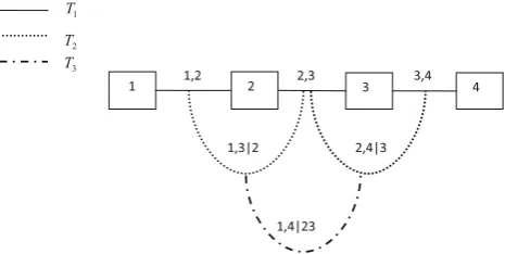
Here,is the symmetric difference operator, and # is the cardinality operator. A regular vine (called D-vine) on 4 vari-ables is exemplified in Fig.1.
In Fig.1,T1 is a tree with nodesN1 = {1,2,3,4}and
edgesE1= {{1,2},{2,3},{3,4}}, andT2is a tree with nodes N2 =E1and edgesE2 = {{1,3|2},{2,4|3}}. For an edge,
1 T
2 T
3 T
[image:2.595.309.542.578.695.2]the set of variables to the right of the vertical slash is called a conditioning set, and the set of variables to the left of the vertical slash is called a conditioned set. The constraint set, conditioning set and conditioned set of an edge are defined as follows.
Definition 2 ∀e = {e1, e2} ∈ Ei (i =2, . . . ,n−1), the
constraint set related to edgeeis the subset of{1, . . . ,n} reachable frome. WriteUe∗for the constraint set ofe. The
conditioning setofeisDe=Ue∗1∩U ∗
e2, and the conditioned set ofeis{Ue∗1\De, U
∗
e2 \De}.
Here,Ue∗1\Derepresents the relative complement ofDein Ue∗1. We might writee˙1forUe∗1 \ De ande˙2forUe∗2 \De. Hence the conditioned set ofeis{˙e1,e˙2}. Throughout the
work, we represent edgeeby{˙e1,e˙2|De}. Referring to Fig.1,
the set of edges for treeT3contains only one element:E3=
{{1,4|2,3}}; the constraint set of the edge is{1,2,3,4}, the conditioned set of the edge is{1,4}, and the conditioning set of the edge is{2,3}. If e = {e1, e2} ∈ E1, we have
Ue∗= {e1, e2}andDeis empty.
Ann-variate copula is ann-variate probability distribution defined on the unit hypercube[0,1]nwith uniform marginal distributions. There is a one-to-one correspondence between the set ofn-variate copulas and the set ofn-variate distribu-tions, as was stated in a theorem bySklar(1959).
Theorem 1 Given random variables X1, . . . ,Xn having
continuous distribution functions F1(x1),· · ·, Fn(xn)and
a joint distribution function F(x1, . . . ,xn), there exists a
unique n-variate copula C(·)such that
F(x1, . . . ,xn)=C(F1(x1), . . . ,Fn(xn)),
∀(x1, . . . ,xn)∈Rn. (1)
And conversely, given continuous distribution functions F1(x1), · · ·, Fn(xn) and an n-variate copula C(·),
F(x1,· · ·,xn)defined through Eq.(1)is an n-variate
dis-tribution with marginal disdis-tribution functions F1(x1), . . .,
Fn(xn).
The coupling of regular vines and bivariate copulas pro-duces a particularly versatile tool, called vine copula or pair-copula construction, for modelling multivariate data. The backbone of vine copula is re-forming, according to the structure of a regular vine, a multivariate copula into a hier-archy of (conditional) bivariate copulas. Given a regular vine
V, for anye∈E(V)with the conditioned set{˙e1,e˙2}and the
conditioning setDe, letXXXe=(Xv:v∈De)denote the
vec-tor of random variables indicated by the conditioning setDe.
Throughout the work, all vectors are defined to be row vec-tors. DefineCe˙1e˙2|De(·)(resp.ce˙1e˙2|De(·)) to be the bivariate
copula (resp. copula density) for the edgee.Ce˙1e˙2|De(·)and ce˙1e˙2|De(·)are conditioned onXXXe. Letxe˙1,xe˙2andxe, respec-tively, denote, from the generic point of view, the value of
Xe˙1,Xe˙2 andXXXe. We have the following theorem (Bedford and Cooke 2001).
Theorem 2 LetV = {T1, . . . ,Tn−1}be a regular vine on
the random variables {X1, . . . ,Xn}, and let the marginal
distribution function Fi(xi) and density function fi(xi) (i = 1, . . . ,n) be given. Then the vine-dependent n-variate distribution is uniquely determined with density function
f(x1, . . . ,xn)= n
i=1
fi(xi)
×
e∈E(V)
ce˙1e˙2|De
uxe, wxe|XXXe=xe
.
Here,uxe = Fe˙1|De(xe˙1| XXXe =xe)andwxe = Fe˙2|De(xe˙2| X
X
Xe = xe)are two conditional marginal distributions, both
conditioned on XXXe. All the involved conditional marginal
distributions can be derived from the marginal distribution functions and copula densities. (See Section 2.2 of the supple-mentary material for more discussion on deriving conditional marginal distributions.) Theorem2 claims that we are able to derive the n-variate density function, once we are given the n marginal distribution functions and all the bivariate copulas originated from the regular vine. The n marginal distribution functions can be readily estimated from col-lected data, either parametrically or empirically, by using standard univariate methods. The estimation of the involved bivariate copulas is, however, non-trivial and still remains an open problem. Note that the form of the copula den-sity ce˙1e˙2|De(·)(namely the dependence structure between Fe˙1|De(Xe˙1| XXXe = xe) and Fe˙2|De(Xe˙2| XXXe = xe)) can be highly influenced by the value of XXXe. The dependence
of the form of ce˙1e˙2|De(·) on XXXe is always intentionally
ignored in the community of vine copula, due to certain practical concerns such as computational load and the curse of dimensionality (see, e.g., Kauermann and Schellhase 2014).
In Sect.3, we will introduce a family of minimally informative copulas that can cope with the dependence of ce˙1e˙2|De(·)onXXXe. Deriving a minimally informative copula involves the notion of relative information (Kullback–Leibler divergence).
2.2 Relative information
I(P|Q)=
log
dP dQ
dP.
Here,ddQP is the Radon–Nikodym derivative ofPw.r.t.Q. If
μis any measure onfor whichddPμ andddQμ exist, then the relative information ofQfrom Pcan be written into
I(P|Q)=
plog
p q
dμ,
where p=ddPμ andq =ddQμ.
Relative information is always nonnegative and is minimized to 0 whenP=Qalmost everywhere.
Relative information is a popular “metric” for measur-ing probability distance. There are two elegant properties of relative information, making it a natural criterion for copula selection. Firstly, relative information is invariant under monotonic transformation. For example, letn-variate distributions f(x1, . . . ,xn) and g(x1, . . . ,xn) have
iden-tical marginal distributions: fi(xi), i = 1, . . . ,n. Write
cf(·) for the copula density of f(x1, . . . ,xn), and cg(·)
for the copula density of g(x1, . . . ,xn). If we want to
approximate
f(x1, . . . ,xn)= n
i=1
fi(xi)cf (F1(x1), . . . ,Fn(xn)) ,
by
g(x1, . . . ,xn)= n
i=1
fi(xi)cg(F1(x1),· · · ,Fn(xn)) ,
then we have
I(f|g)=
Rn f(x1, . . . ,xn)log
f(x1, . . . ,xn)
g(x1, . . . ,xn)
dx1· · ·dxn
=
Rn
cf(F1(x1), . . . ,Fn(xn))log
cf(F1(x1), . . . ,Fn(xn))
cg(F1(x1), . . . ,Fn(xn))
dF1(x1)· · ·dFn(xn). (2)
Therefore, if f(x1, . . . ,xn)is the true law andcg(F1(x1), . . ., Fn(xn)) has the minimum relative information w.r.t.
cf(F1(x1),. . .,Fn(xn)), theng(x1, . . . ,xn)has the minimum
relative information w.r.t. f(x1, . . . ,xn). In what follows,
we say an n-variate copula is minimally informative if the relative information of it from the independence cop-ula is minimal. Therefore, a minimally informative copcop-ula
is the most “independent” copula among all the qualified copulas. See (Jaynes 2003, Chapter 11) for an enlight-ening explanation on relative information (therein called entropy), which gives justification for the employment of minimally informative copulas for analyzing multivariate data. Given a multivariate data set, Eq. (2) reduces the problem of finding the minimally informative multivariate distribution to the problem of finding the minimally infor-mative multivariate copula. Then, how to find the minimally informative multivariate copula? The second property of rel-ative information claims that a vine-dependent distribution is minimally informative if and only if all its bivariate cop-ulas are minimally informative (Bedford and Cooke 2002). Therefore, to guarantee that a multivariate copula be min-imally informative, we only need to find the minmin-imally informative bivariate copula for each edge in the regular vine.
We now frame our line of approach to modelling multi-variate data as follows. Given a multivariate data set and a regular vine on the involved random variables, we will formulate the optimal bivariate copula for every edge in the regular vine from the top level to the bottom level. A bivariate copula is optimal in the sense that it meets all the specified constraints and is minimally informative, making the corresponding multivariate copula minimally informative. Clearly, there are two problems related to our approach, which will be attended to in the following sec-tion: (1) the type of constraints that a bivariate copula needs to meet and (2) how to analytically formulate the optimal copula.
Remark 1 Here, we presume that the structure of the regular vine is given. The determination of the structure of a regular vine is an open topic of great importance. A well-structured vine copula can capture the underlying multivariate law by copulas in the lower hierarchy of the vine and therefore can reduce computational load and mitigate the curse of dimen-sionality by simplifying copulas in the deeper hierarchy of the vine (Dißmann et al. 2013). This topic is beyond the scope of the current work and will be addressed in the future.
3 Minimally informative copula
In the following, for exposition convenience, we assume that thenrandom variablesX1,. . .,Xnare uniformly distributed.
Example 1 LetV= {T1, . . . ,Tn−1}be a regular vine on the
uniform random variables{X1, . . . ,Xn}. For now, we
con-centrate on an edgee ∈ E1; that is, the conditioning set of eis empty. Let Xi and Xj (1 ≤ i < j ≤ n) be the two
uniform random variables joined by the edgee. A bivariate copula densityc¨e(xi,xj)for the edgeeis said to be
qual-ified, if the followingk (≥ 1) expectation constraints are satisfied:
α=
1
0
1
0
h(xi,xj)c¨e(xi,xj)dxidxj, =1, . . . ,k.
(3)
Here, the real-valued functionsh1(xi,xj), . . . ,hk(xi,xj)are
linearly independent, modulo the constants;{α1, . . . , αk}are
known, whose values can be obtained from data or expert elicitation. Equation (3) says that a qualified copula should satisfy the constraints that the expected value of the random variableh(Xi,Xj)isα for = 1, . . . ,k. For example,
whenhk(Xi,Xj) = XiXj, then the rank correlation of a
qualified copula should beαk.
In practice, we know a priori the expected values of the random variables{h1(Xi,Xj), . . . ,hk(Xi,Xj)}; then,
every qualified copula for edge e should satisfy the con-straints given in Eq. (3), and we select from these qualified copulas the minimally informative one. Many constraints can be written in the form of expectation constraints. For example, constraints are commonly specified in the form of probabilities. Yet, a probability can be expressed as the expectation of an identity function. Another conven-tional way to specify constraints is in the form of various kinds of correlations, such as product-moment correlations. Yet, due to the one-to-one correspondence between the set of n-variate copulas and the set of n-variate distribu-tions, any correlation can be expressed as an expectation w.r.t. an appropriate copula. The way of specifying expec-tation constraints also allows a wider range of constraints if desired.
Another major advantage of specifying expectation con-straints is that the minimally informative bivariate copula for an edge, satisfying all the specified expectation constraints, can be readily determined.
Example 2 (continued) According toNussbaum(1989) and
Borwein et al.(1994) (seeBedford and Wilson(2014) for a summary), there exists uniquely a minimally informative bivariate copula satisfying all the expectation constraints in (3) with the copula density given by
ˆ
ce(xi,xj)=d1(xi)d2(xj)exp
λ1h1(xi,xj)+ · · · +λkhk(xi,xj)
. (4)
The Lagrange multipliers λ1, . . . , λk are unknown and
depend nonlinearly onα1, . . . , αk. The functionsd1(·)and
d2(·)are two regularity functions, makingcˆe(xi,xj)a copula
density. LetA(xi,xj)denote the exponential part:
A(xi,xj)=exp
λ1h1(xi,xj)+ · · · +λkhk(xi,xj)
.
Though A(xi,xj) has a closed-form expression, the two
regularity functions don’t. Hence,cˆe(xi,xj)need to be
deter-mined numerically. (See Section 1 of the supplementary material for the determination of the two regularity functions and the Lagrange multipliers.)
LetCCC([0,1]2)denote the space of continuous functions defined on the unit square [0,1]2. Though cˆe(xi,xj) is
minimally informative, it may not well approximate the underlying true copula densityce(xi,xj). We want to
approx-imatece(xi,xj)bycˆe(xi,xj)to any required degree, which
is accomplished by letting h1(xi,xj), . . . ,hk(xi,xj) be
elements of a particular basis for the spaceCCC([0,1]2). Specif-ically, defineC(f)by
C(f)=ce˙1e˙2|De(·): ∀e∈E(V) .
Namely, C(f) is the set of all possible bivariate cop-ula densities originated from the multivariate distribution f(x1, . . . ,xn)and therefore is infinite. Furthermore, define L(f)by
L(f)= {log(c):c∈C(f)}
=log(ce˙1e˙2|De(·)): ∀e∈E(V) .
It has been proved by Bedford et al. (2016) that the set
C(f)(and thereforeL(f)) is relatively compact in the space C
C
C([0,1]2). Therefore, by selecting sufficiently many basis functions,{h1(xi,xj),. . .,hk(xi,xj)}, from a particular basis
for the spaceCCC([0,1]2), we can approximate log(ce(xi,xj))
to any required degree (>0)by a linear combination of h1(xi,xj),. . .,hk(xi,xj):
sup
(xi,xj)∈[0,1]2
||logce(xi,xj)
−λ1h1(xi,xj)− · · · −λkhk(xi,xj)||< .
Thencˆe(xi,xj)defined in Eq. (4) shall well approximate the
true copula densityce(xi,xj). Here, the metric employed on
the spaceCCC([0,1]2)is the sup norm, hence only requiring the continuity ofce(xi,xj).
For later reference, we call the set of basis functions
{h1(xi,xj), . . . ,hk(xi,xj)} as “information set.” We
spaceCCC([0,1]2). Let{h1(·), . . . ,hk(·), . . .}be a countable
set of basis functions that span the spaceCCC([0,1]2). Then for any copula density in C(f) and any required level , we can select from{h1(·), . . . ,hk(·), . . .}finite appropriate
basis functions whose linear combination can approximate the copula density to the required level. However, the resulted linear combination is not minimally informative. Then we turn back to the logarithmic counterpart ofC(f), i.e., L(f). Due to the one-to-one correspondence, L(f) is also a relatively compact set in the space CCC([0,1]2). Therefore, for any element in L(f) and any required level δ(>0), we can select from {h1(·), . . . ,hk(·), . . .}
finite appropriate basis functions whose linear combina-tion can approximate the element to the required level δ. By the theoretical work given in Nussbaum (1989) and
Borwein et al. (1994), we are able to derive the mini-mally informative copula density from the linear combi-nation, i.e., Eq. (4). The derived minimally informative copula density well approximates the true underlying cop-ula density.
There are many bases for the space CCC([0,1]2), e.g.,
{xipxqj : p,q ≥ 0}. Note that we are not selecting basis functions from a whole basis, which is impossible and unnecessary. We are indeed selecting from a finite set, e.g.,
{xipxqj : 0 ≤ p,q ≤ r}with an appropriate power limit r. Theoretically, by lettingk be sufficiently large, we can well approximate any copula density inC(f)by the same information set{h1(xi,xj),. . .,hk(xi,xj)}. However, more
basis functions will bring about moreλ’s to be estimated and, consequently, more computational load. Hence, when approximating an individual copula density, we can deter-mine the entry of a basis function into the information set according to its contribution to the approximation. Specifi-cally, let{(xi(v),x(v)j ) :1 ≤ v ≤ m}denote a sample ofm data points fromce(xi,xj). Let Bdenote a finite set of
can-didate basis functions, e.g., B = {xipxqj : 0 ≤ p,q ≤ r}. The procedure for selecting basis functions is outlined in Algorithm1.
Algorithm 1Information Set Determination 1: Set the information set to be empty.
2: Select fromBthe basis function that yields the largest value of the log-likelihood
m
v=1
log(cˆe(xi(v),x(v)j )). (5)
3:whilethe stopping criterion is not metdo
4: Move the selected basis function fromBinto the information set. 5: Select fromBthe basis function which, together with the basis functions in the information set, yields the largest value of the log-likelihood (5).
6:end while
For ease of exposition, in what follows, we refer the log-likelihood from fitting a minimally informative copula to a data set as “estimated likelihood” and refer the log-likelihood from fitting the true underlying copula to a data set as “true log-likelihood.” We should note the following points.
– The stopping criterion in Algorithm 1 could be the maximal number of basis functions or the minimal improvement in the estimated log-likelihood. By adding a new basis function to the information set, the esti-mated log-likelihood will always increase. Hence, there is no optimal number of basis functions. The choice of the number of basis functions involves the trade-off between approximation accuracy and computational load.
– Selecting basis functions according to the estimated log-likelihood is in consistent with information mini-mization. It is well known that the values of the Lagrange multipliers λ ( = 1, . . . ,k), satisfying the expecta-tion constraints, are also maximum likelihood estimates (see, e.g.,Barron and Sheu 1991).
A distinguishing feature of our approach is that we have made no assumption on the structure of the underlying multivariate distribution f(x1, . . . ,xn), except that all the
(conditional) bivariate copulas should be continuous. The expectation constraints are extracted from available data or expert judgement, and will be further studied in the following section.
4 Conditional copula approximation
For the practical implementation of our approach, one fun-damental problem needs to be solved: how to evaluate
{α1, . . . , αk}according to the data at hand. In Sect.3, we took,
for example, an edge inE1. Therein,α (=1, . . . ,k) can be readily evaluated by calculating the sample mean of the random variableh(Xi,Xj). For example, ifhk(Xi,Xj)=
XiXj, thenαkcan be approximated by the sample mean of
XiXj:αk =m1
m
v=1xi(v)x
(v)
j .It should be noted that for an
edgeein treeTi(i =2, . . . ,n−1), the conditioning setDeis
no longer empty. For notational simplicity, we defineUxe = Fe˙1|De(Xe˙1|XXXe=xe)andWxe=Fe˙2|De(Xe˙2|XXXe=xe). Let uxe (resp.wxe) denote the generic value ofUxe (resp.Wxe).
The expectation constraints now should take into account the value ofXXXe:
α(xe)=
1
0
1
0
ce˙1e˙2|De
uxe, wxe|XXXe=xe
0.0 0.2 0.4 0.6 0.8 1.0
0.0
0
.2
0.4
0.6
0.8
1.0
xe(
v)
hl
(
uxe
(
v
), w
xe
(
v
))
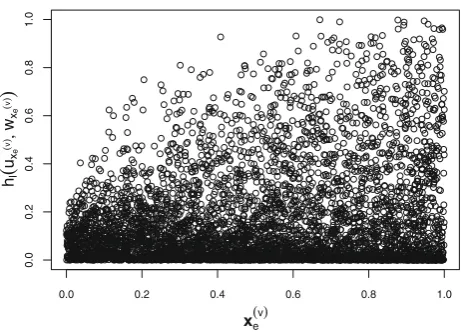
Fig. 2 An illustrative scatter plot of{(x(v)e , h(ux(v)
e , wx(v)e )) : 1 ≤
v≤5000}
Clearly,α(·)is now a function ofXXXe—the conditioning
ran-dom vector related to the edgee. If, at a point XXXe = xe,
we have a sizable sample of(Uxe,Wxe), we intuitively
esti-mate α(xe)by the sample mean of the random variable
h(Uxe,Wxe). Furthermore, if there are sufficiently many
realizations of the conditioning vector—conditioned on each of which we have a sizable sample of (Uxe,Wxe)—we
will be able to approximate the functional form ofα(XXXe),
which is a classical regression problem. Apparently, col-lected real-life data will never be what we are fancying here. Because {X1, . . . ,Xn} are continuous random
vari-ables, for any point XXXe = xe, there will be only one
realization of the random variable h(Uxe,Wxe). We
cer-tainly cannot replace “estimatingα(xe)by the sample mean
ofh(Uxe,Wxe)” with “estimatingα(xe)by one realization
of h(Uxe,Wxe).” One simple explanation is that we
con-ventionally treat a realization of a random variable as the mode of the distribution of that random variable (e.g., when conducting maximum likelihood estimation). The mean and the mode of a distribution usually take different values, and the relationship between them changes from distribution to distribution. As stated in “Appendix,” under some mild assumptions,α(xe)(and, therefore, the Lagrange
multipli-ers{λ1, . . . , λk}) is a continuous function ofxe. One may
suggest to approximate such function by fitting a regression model to the data{(x(v)e , h(ux(v)
e , wx(v)e )): 1 ≤ v ≤ m}
(with {xe(v): 1 ≤ v ≤ m} being the predictors).
How-ever, the fact is that there is no deterministic relationship betweenh(ux(v)
e , wx(v)e )andx
(v)
e ; the scatter plot of the data {(x(v)e , h(ux(v)
e , wx(v)e )):1 ≤ v ≤ m}is rather erratic (see
Fig.2).
We have to come up with an efficient surrogate for the sample mean of the random variableh(Uxe,Wxe).
Bedford et al.(2016) approached the above problem by dividing the domain ofXXXeinto equal-volume subregions and
assuming that the copula densityce˙1e˙2|De(·)dose not change
when XXXe varies within an individual subregion. Evidently,
their approach suffers from certain inherent drawbacks. For example, the partition of the domain of XXXe is rather
sub-jective. Even if they divide the domain by using, say, the CART (classification and regression tree), the fitted copula density is still not appealing: It is bumpy. In the following, we propose to relax the conditional expectation (6) and com-pute an average over a neighborhood of XXXe = xe, which
is achieved by invoking the kernel-regression technique; see (Hastie et al. 2009, Chapter 6) for a brief introduction on kernel regression. Compared with parametric methods, ker-nel smoothing methods have the advantage that they make relatively milder structural assumptions. By employing ker-nel smoothing methods, two approximations are happening here:
– expectation is approximated by averaging over sample data;
– conditioning at a point is relaxed to conditioning on a region encircling that point.
Remark 2 Note that Eq. (6) provides a method to test if the simplifying assumption can be employed for a particular edge. Specifically, if the simplifying assumption holds, then the conditional copulace˙1e˙2|De
uxe, wxe|XXXe=xe
does not depend on the value of XXXe. Therefore,α(xe)should be a
constant:
α=
1
0
1
0
ce˙1e˙2|De
uxe, wxe
h(uxe, wxe)duxedwxe.
Hence, for each value of XXXe = xe, we calculateα(xe).
Ifα(xe)is constant (or varies within a small range), then
we might employ the simplifying assumption. Otherwise, if
α(xe)varies within a wide range or demonstrates an obvious
relationship withxe, then we cannot employ the simplifying
assumption.
4.1 Weighted average and weighted linear regression
For an edge e ∈ Ei (2 ≤ i ≤ n − 1), Xe˙1 and Xe˙2 are the two conditioned random variables, and XXXe is the conditioning random vector (having (i − 1) ele-ments). Let (xe(v)˙1 , xe˙(v)2 , x(v)e ) denote the vth realization
of (Xe˙1, Xe˙2, XXXe) for v = 1, . . . ,m. We now approx-imate the conditional expectation of the random variable h(Uxe, Wxe), for 1≤≤kand an arbitrary pointXXXe=xe.
LetKμ(xe, x)be a kernel function, allocating an
appro-priate weight tox(∈ [0,1]i−1) according to its distance from xe. For example, the radial Epanechnikov kernel is defined
[image:7.595.55.286.52.218.2]Kμ(xe, x)=D ||
xe−x|| μ
,
in which|| · ||is the Euclidean norm, and
D(z)=
3(1−z2)/4, if|z|<1;
0, otherwise.
Here, the parameterμ(>0), controlling the range of the local neighborhood, is usually called the bandwidth or window width. (Section 2.2 of the supplementary material discusses the high-dimensional problem for local learning methods.) The normal kernel with D(z) = φ(z)is another popular kernel, where φ(z) is the standard normal density func-tion. The radial Epanechnikov kernel is optimal in terms of mean squared error (Epanechnikov 1969), while the nor-mal kernel is more mathematically tractable. Intuitively, we can approximate α(xe) by the Nadaraya–Watson
kernel-weighted averageαˆ(xe, μ):
ˆ
α(xe, μ)=
m
v=1Kμ(xe, x(v)e )h(ux(v)
e , wxe(v))
m
v=1Kμ(xe, xe(v))
, (7)
in whichux(v)
e =Fe˙1|De(x
(v)
˙
e1 |XXXe=x
(v)
e )andwx(v)
e =Fe˙2|De
(x(v)e˙
2 | XXXe = x
(v)
e ). The weighted average αˆ(xe, μ) puts
more weight on the data points that fall within distanceμ fromxe.
One drawback of locally weighted average is that it can be biased approaching the boundary of the domain of XXXe,
because of the asymmetry of the data near the boundary. Locally weighted linear regression can help reduce bias dra-matically at a modest cost in variance (Fan 1992). It exploits the fact that, over a small enough subset of the domain, any sufficiently nice function can be well approximated by an affine function. (See “Appendix” for the continuity and dif-ferentiability of the functionα(·).)
However, locally weighted linear regression cannot be directly applied here, because it may return an imprac-tical estimate of α(xe). We take the polynomial basis {xipxqj: p,q ≥ 0}, for example. For any basis function from the polynomial basis, the value of the conditional expectation α(xe) should falls within the interval (0,1).
However, locally weighted linear regression cannot guaran-tee that its estimate falls into the interval(0,1). To avoid impractical estimates, we put an inequality restriction on regression coefficients. The inequality-constrained weighted linear regression approach to approximating α(xe)
pro-ceeds as follows. Let θθθ = (θ0, θ1, . . . , θi−1)be a vector
of coefficients. At any pointXXXe = xe, solve the following
inequality-constrained least-square problem:
ˆ
θθθ(xe, μ)=arg min
θθθ
m
v=1
Kμ(xe, x(v)e )
×h(ux(v)
e , wx(v)e )−(1, x
(v)
e )θθθtr 2
,
subject to 0 < (1, xe)θθθtr < 1.Here, “tr” is the transpose
operator. Then the optimal estimate ofα(xe)is
ˆ
α(xe, μ)=(1, xe)θθθ(ˆ xe, μ)tr. (8)
Guaranteed by the additional constraint, the estimate
ˆ
α(xe, μ) will always be practical. The estimateθθθ(ˆ xe, μ)
can be calculated by Dantzig–Cottle algorithms (Cottle and Dantzig 1968). According to Theorem 1 ofLiew (1976), it is easy to prove that, when m is sufficiently large, the inequality-constrained least-square problem will reduce to a non-constrained least-square problem. Note that though we fit a linear model to the data within the neighborhood of X
X
Xe =xe, we only utilize the fitted linear model to evaluate ˆ
α(xe, μ) at the single point XXXe = xe. Apparently,
com-pared with locally weighted average, inequality-constrained locally weighted linear regression is more computationally demanding.
Like any local learning problem, one needs to determine the optimal range of the neighborhood, i.e., the value of
μ. A variety of automatic, data-based methods have been developed for optimizing the bandwidth, with the general consensus that the plug-in technique (Sheather and Jones 1991) and cross-validation technique (Rudemo 1982) are the most powerful; see Köhler et al. (2014) for a recent review. Plug-in methods require subjective estimators of certain unknown functions and perform badly in multivari-ate regression. Hence, we here illustrative the leave-one-out cross-validation approach to determining the optimal band-widthμ. For five- or tenfold cross-validation, the appropriate translations are obvious.
For an edgee∈Ei(2≤i ≤n−1), given the data{(x(v)e˙1 ,
xe(v)˙ 2 ,x
(v)
e ):1 ≤ v ≤ m}, we in turn approximateα(xe(v))
for 1 ≤ v ≤ m. For a particularv and given the informa-tion set{h1(u, w), . . . ,hk(u, w)}, utilize the remaining data {(xe(˙1j), xe˙(2j), xe(j)):1 ≤ j = v≤ m}and Eqs. (7) or (8) to
calculate the estimate ofα(x(v)e ), denoted byαˆ(x(v)e , μ)for =1, . . . ,k. According to{ ˆα1(x(v)e , μ),· · ·,αˆk(xe(v), μ)},
we can readily approximate the true copula densityce˙1e˙2|De (u, w|XXXe =x(v)e )bycˆe˙1e˙2|De
u, w|XXXe=x(v)e ; μ
:
ˆ ce˙1e˙2|De
u, w|XXXe=x(v)e ; μ
=d1(v)(u;μ)d2(v)(w;μ)
×exp
λ(v)1 (μ)h1(u, w)+ · · · +λ(v)k (μ)hk(u, w)
where the two regularity functions, d1(v)(u;μ) and d2(v)(w;μ), and the Lagrange multipliers {λ(v)1 (μ), . . .,
λ(v)k (μ)}are all calculated in the manner of Section 1 in the
supplementary material.
The optimal bandwidth for edgee, denoted byμ∗e˙ 1e˙2|De,
is
μ∗ ˙
e1e˙2|De =arg maxμ m
v=1
log
ˆ ce˙1e˙2|De
ux(v)
e , wx(v)e |XXXe=x
(v)
e ; μ
.
Note that the optimal bandwidths for different edges are dif-ferent.
4.2 Basis function selection for conditional copulas
Recall that for an unconditional copula, we select from B the basis function that most improves the log-likelihood (5); if we havem data points, then the log-likelihood is a summation ofm elements. However, for each conditional copula, the corresponding log-likelihood contains only one element. For example, if we have data{(xe(v)˙
1 , x
(v)
˙
e2 , x
(v)
e ) :
1 ≤ v ≤ m} for edge e, then we will have m dif-ferent conditional copulas: ce˙1e˙2|De
u, w|XXXe =x(v)e
, for 1 ≤ v ≤ m. Of all the m data points {(ux(v)
e , wx(v)e ) :
1 ≤ v ≤ m}, only the datum (ux(v)
e , wx(v)e ) comes from
the conditional copula ce˙1e˙2|De(u, w| XXXe = x
(v)
e ).
There-fore, the estimated log-likelihood contains only one element: log(cˆe˙1e˙2|De(ux(v)
e , wx(v)e | XXXe = x
(v)
e ;μ)). If we select basis
functions for ce˙1e˙2|De
u, w|XXXe=x(v)e
according to the estimated log-likelihood, then the selected basis functions are optimal only in terms of the single datum(x(v)e˙
1 ,x
(v)
˙
e2 ,x
(v)
e ).
Consequently, the approximating copulacˆe˙1e˙2|De(u, w|XXXe=
x(v)e ;μ) will be overfitting. Another problem related to
selecting basis functions for conditional copulas is the huge computational load. If we are dealing with ann-variate vine copula, then we will have to approximatem× (n−1)(2n−2) conditional bivariate copulas. Even worse, taking account of cross-validation, if we determine the optimal value ofμ among, say, a set of 100 values, then the computational load is 100×m×(n−1)(2n−2).
To alleviate the above-mentioned two problems, we here develop a two-stage procedure for approximating all the con-ditional copulas related to an edgee∈Ei (2 ≤i ≤n−1);
see Algorithm2.
Algorithm 2Two-Stage Procedure 1:procedureStage One
2: Divide the domain ofXXXeintozregions:[0,1]i−1=R1∪R2∪ · · · ∪Rz.
3: Divide the data{(u
x(v)e , wx(v)e ) : 1 ≤ v ≤ m}intozsubsets: {(ux(v)
e , wx(v)e ):x
(v)
e ∈Rj,1≤v≤m}, j=1, . . . ,z.
4: forj=1, . . . ,zdo
5: Treat the data{(u
x(v)e , wx(v)e ) : x
(v)
e ∈ Rj,1 ≤ v ≤m}as
coming from an unconditional copula and determine the information set, denoted byBj, for them by using Algorithm1.
6: end for 7:end procedure 8:procedureStage Two
9: Letμdenote the value of the bandwidth. 10: for1≤v≤mdo
11: Ifx(v)e ∈Rj, then the information set used for approximating
the conditional copulace˙1e˙2|De(u, w|XXXe=x(v)e )isBj.
12: Use a local learning method to calculate
{ ˆα1(x(v)e , μ), . . . ,αˆk(x(v)e , μ)}, wherek=#Bj.
13: Use the method developed in Section 1 of the supplementary material to calculate the Lagrange multipliers{λ(v)1 (μ),· · ·,λ(v)k (μ)} and numerically determine the two regularity functionsd(v)1 (u;μ)
andd2(v)(w;μ).
14: The minimally informative copula for
ce˙1e˙2|De
u, w|XXXe=xe(v)
is ˆ
ce˙1e˙2|De
u, w|XXXe=x(v)e ;μ
=d1(v)(u;μ)d2(v)(w;μ)
exp
λ(v)1 (μ)h1(u, w)+ · · · +λ(v)k (μ)hk(u, w)
,
where{h1(u, w), . . . ,hk(u, w)}are the basis functions inBj.
15: end for 16: Calculate
m
v=1
logcˆe˙1e˙2|De
ux(v)
e , wx(v)e |XXXe=x
(v)
e ;μ
. (9)
17: Repeat steps 9–16 for different values ofμand select the optimal one that maximizes the estimated log-likelihood (9).
18:end procedure
We should note the following points.
– The two-stage procedure utilizes the continuity ofce˙1e˙2|De (u, w| XXXe = xe)onxe. According to Appendix A, the
dependence structurece˙1e˙2|De (u, w|XXXe =xe)changes
continuously withxe. Therefore, for a small region, we
– For a conditional copula in tree T2, it has only one
conditioning variable. Since every individual variable is uniformly distributed, we can divide the domain (i.e., the [0, 1] interval) into a few equal-length subintervals. For a conditional copula in treeTi (i ≥ 3), the elements of
the conditioning random vector are mutually dependent. Instead of subjectively dividing the domain of XXXe into
z regions, we can employ k-means clusteringto parti-tion the observaparti-tions{x(v)e :1≤v≤m}intozclusters,
such that the within-cluster distance is minimized and the between-cluster distance is maximized; see, e.g., Har-tigan and Wong (1979). The “kmeans” function in R software serves this purpose.
– If parallel computing is possible, Stage Two can be cal-culated parallel on each tree level.
5 Numerical study
In this section, we examine the performance of the two-stage procedure via simulated data. Due to lack of space, a real data set is analyzed in the supplementary material.
For illustrative purpose, we focus on the D-vine structure of 6 random variables, with the nodes in treeT1 from left
to right being labeled by{X1,X2,X3,X4,X5,X6}. All the
bivariate copulas originated fromf(x1, . . . ,x6)are from the
same family. For example, all the bivariate copulas originated from a 6-variatet-copula aret-copulas and have the same degrees of freedom.
Three types of bivariate copulas are examined: the Gaus-sian copula, t-copula and Gumbel copula. The Gaussian copula and t-copula are able to model moderate and/or
heavy tails; the Gumbel copula is able to capture asymmetric dependence. In terms of tail dependence, the Gaussian cop-ula is neither lower nor upper tail dependent; the t-copula is both lower and upper tail dependent; the Gumbel cop-ula is upper tail dependent. Due to lack of space, we here only present simulation results of thet-copula. Simulation results of the other copulas are given in the supplementary material. The bivariatet-copula withυ(>2) degrees of free-dom is given byCρ,υ(u, w)=tρ,υ(tυ−1(u),tυ−1(w)),where tυ(·)is the cdf of the one-dimensionalt-distribution withυ degrees of freedom, and tρ,υ(·) is the cdf of the bivariate t-distribution withυ degrees of freedom and correlationρ
∈ (−1,1). The superscript “−1” denotes the inverse of a function.
The parameter setting for simulating data is described as follows. For the five bivariatet-copulas in treeT1, the
correla-tion parameterρtakes in turn (from left to right) the following five values:{0.3,0.4,0.5,0.6,0.7}, which indicates that the dependence structure evolves from weak dependence to strong dependence. All the bivariatet-copulas have 3 degrees of freedom. For a conditional bivariatet-copula related to an edgee, the correlation parameter and the conditioning vari-ables have the following relation:
ρ(xe)=1.4×(x¯e−0.5), (10)
in whichx¯e is the average of the values of the
condition-ing variables. Consequently,α(xe)is differentiable. Under
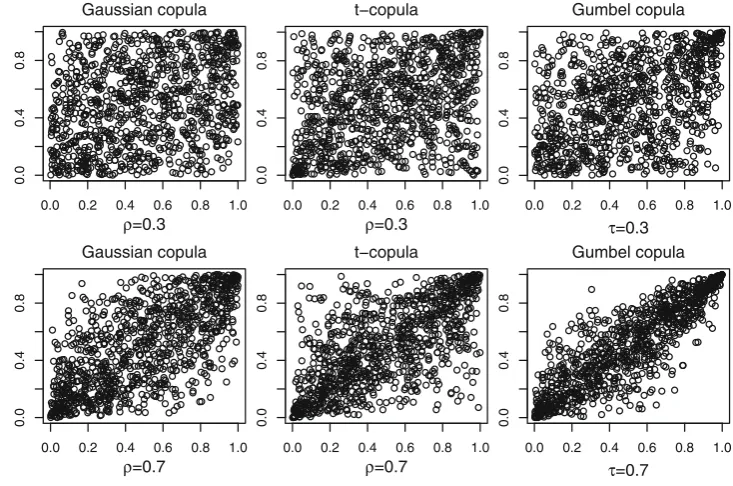
the above parameter setting, we randomly simulate a sample of 1000 data points from the 6-variatet-copula. The scatter plots for copulasc12(u, w)andc56(u, w)are given in Fig.3,
in which scatter plots for two Gaussian copulas and two
Gum-Fig. 3 Scatter plots of samples with size 1000 from different bivariate copulas
0.0 0.2 0.4 0.6 0.8 1.0
0.0
0.4
0.8
ρ=0.3 Gaussian copula
0.0 0.2 0.4 0.6 0.8 1.0
0.0
0.4
0.8
ρ=0.3 t−copula
0.0 0.2 0.4 0.6 0.8 1.0
0.0
0.4
0.8
τ=0.3 Gumbel copula
0.0 0.2 0.4 0.6 0.8 1.0
0.0
0.4
0.8
ρ=0.7 Gaussian copula
0.0 0.2 0.4 0.6 0.8 1.0
0.0
0.4
0.8
ρ=0.7 t−copula
0.0 0.2 0.4 0.6 0.8 1.0
0.0
0.4
0.8
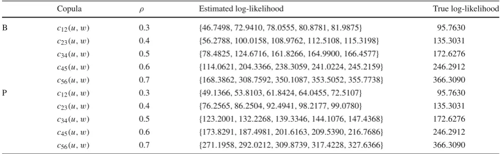
[image:10.595.177.544.473.716.2]Table 1 The evolution of the estimated log-likelihood by gradually adding basis functions:t-copula
Copula ρ Estimated log-likelihood True log-likelihood
B c12(u, w) 0.3 {46.7498,72.9410,78.0555,80.8781,81.9875} 95.7630
c23(u, w) 0.4 {56.2788,100.0158,108.9762,112.5108,115.3198} 135.3031
c34(u, w) 0.5 {78.4825,124.6716,161.8266,164.9900,166.4577} 172.6276
c45(u, w) 0.6 {114.0621,204.3366,238.3059,241.0224,245.2159} 246.2912
c56(u, w) 0.7 {168.3862,308.7592,350.1087,353.5052,355.7738} 366.3090 P c12(u, w) 0.3 {49.1366,53.8103,61.8424,64.0455,72.5107} 95.7630
c23(u, w) 0.4 {76.2565,86.2504,92.4941,98.2177,99.0780} 135.3031
c34(u, w) 0.5 {123.2001,132.2268,139.3346,144.1076,147.4368} 172.6276
c45(u, w) 0.6 {173.8291,187.4981,201.6163,209.5390,216.7686} 246.2912
c56(u, w) 0.7 {271.1958,292.0212,309.8739,317.4228,327.6366} 366.3090
bel copulas are also included.τ represents the Kendall rank correlation coefficient. Figure3shows that, whenρ=0.3 or
τ =0.3, the simulated data do not have an evident pattern; whenρ=0.7 orτ =0.7, the relation between the involved two random variables is noticeable from the data.
Two different bases are used to construct two differ-ent families of minimally informative copulas: the Bern-stein basis functions,6pup(1−u)6−pq6wq(1−w)6−q : 0≤ p,q ≤6 , and the polynomial basis functions{upwq : 0 ≤ p,q ≤ 6}. Here the polynomial degree is 6. (Via intensive simulation study, we found that increasing the power to larger than 6 will improve a little the approxi-mation, but will impose a lot of additional computational load.) Although we can approximate a bivariate copula to any required degree, given only a finite set of candidate basis functions, different bases will have different efficiency. Hence, we want to compare Bernstein basis with the poly-nomial basis.
We now approximate the five bivariate copulas in treeT1
by minimally informative copulas. The estimated and true log-likelihoods are summarized in Table1.
In Table1, rows 2–6 stand for approximating the five copulas by Bernstein basis functions, and rows 7–11 stand for approximating the same five copulas by polynomial basis functions. For example, when approximatingc12(u, w),
the estimated log-likelihood after selecting the first opti-mal Bernstein basis function (resp. polynomial basis func-tion) is 46.7498 (resp. 49.1366). After adding the second optimal Bernstein basis function (resp. polynomial basis function), the estimated log-likelihood increases to 72.9410 (resp. 53.8103). After selecting five Bernstein basis func-tions (resp. polynomial basis funcfunc-tions), the final estimated likelihood is 81.9875 (resp. 72.5107), while the true log-likelihood is 95.7630. It is observed from Table1 that, for Bernstein basis, the joining of the fifth basis function does not contribute much to the estimated log-likelihood. In Table1,
for each edge, the estimated log-likelihood with five Bern-stein basis functions is larger than that with five polynomial basis functions. Indeed, for each edge, the estimated log-likelihood with three Bernstein basis functions is already larger than that with four polynomial basis functions, show-ing the competence of Bernstein basis.
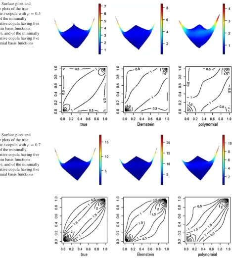
Surface plots and contour plots for copulasc12(u, w)and
c56(u, w)are drawn in Figs.4and5.
In Fig.4(resp., Fig.5), the left two panels are the surface plot and contour plot for the true bivariatet-copulac12(u, w)
(resp.,c56(u, w)); the middle two panels are the surface plot
and contour plot for the minimally informative copula hav-ing five Bernstein basis functions; the right two panels are the surface plot and contour plot for the minimally informa-tive copula having five polynomial basis functions. Figures4
and5show that, compared with the minimally informative copula having polynomial basis functions, the minimally informative copula having Bernstein basis functions bears a stronger resemblance with the true copula. Simulation results in the supplementary material also verified that Bernstein basis is more efficient than polynomial basis. Moreover, it is found that a combination of four Bernstein basis functions is capable of producing a good approximation. Hence, in the following, only Bernstein basis is used, and the cardinality of the information set for a conditional copula is set to be four.
We simulate another sample of 1000 data points from the 6-variate D-vine t-copula and approximate the five bivariatet-copulas in treeT1by minimally informative
cop-ulas having five Bernstein basis functions selected from
6
p
up(1−u)6−p6qwq(1−w)6−q:0≤ p,q ≤6
. For each t-copula in tree T1, we calculate the correlation
Fig. 4 Surface plots and contour plots of the true bivariatet-copula withρ=0.3 (left), of the minimally informative copula having five Bernstein basis functions (middle), and of the minimally informative copula having five polynomial basis functions (right)
Fig. 5 Surface plots and contour plots of the true bivariatet-copula withρ=0.7 (left), of the minimally informative copula having five Bernstein basis functions (middle), and of the minimally informative copula having five polynomial basis functions (right)
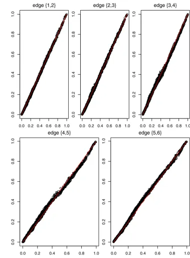
integration. We denote such a value by ρ¯. Apparently, if the minimally informative copula well approximates the true copula, the two sample values,ρˆandρ¯, should be close. We repeat the above procedure for 100 times and obtain, for each t-copula in tree T1, two sequences:{ ˆρi : i = 1,· · ·,100}
and{ ¯ρi :i =1, . . . ,100}. We plot them in Fig.6, in which
the five colors {“black,” “red,” “blue,” “green,” “purple”}, respectively, correspond to the fivet-copulas having
correla-tion coefficients {0.3, 0.4, 0.5, 0.6, 0.7}. Solid lines represent the sequence{ ¯ρi :i =1, . . . ,100}, and dotted lines
repre-sent the sequence{ ˆρi :i =1, . . . ,100}. It is observed from
Fig.6that, for eacht-copula, the two sample valuesρˆi and ¯
ρi are close to each other, showing the competence of the
minimally informative copula.
We now approximate the conditional copulas in tree T2
[image:12.595.75.545.52.576.2]0 20 40 60 80 100
0.2
0.3
0.4
0.5
0.6
0.7
repetition number
P
e
arson correlation coefficient
Fig. 6 Evolving paths of the five sequences{ ˆρi : i = 1, . . . ,100}
(dotted lines) and of the five sequences{ ¯ρi :i =1, . . . ,100}(solid lines). (Color figure online)
are 1000 data points, there will be 1000 × 4 different conditional copulas. Separately determining the informa-tion set for each of them is time consuming and may result in overfitting. Hence, we divide the [0,1] interval into four subintervals:[0,1/4), [1/4,2/4),[2/4,3/4)and
[3/4,1]. For an edge, e.g., {1,3|2}, we group the data
{(F1|2(x1(v)|x2(v)),F3|2(x3(v)|x2(v))):1≤v≤1000}into four
subsets, respectively, corresponding tox2(v)falling into subin-tervals [0,1/4), [1/4,2/4), [2/4,3/4) and[3/4,1]. Then we employ Algorithm2to approximate each of the 1000×4 conditional copulas. To determine the optimal value ofμ, we select it from a set of 10 candidates:{0.1,0.2, . . . ,0.9,1}. The candidate bandwidths are determined to balance the computational load and the approximation accuracy. We
approximate {α1(xe), . . ., αk(xe)} using locally weighted
average.
The total true log-likelihoods for edges{{1,3|2},{2,4|3},
{3,5|4}, {4,6|5}} are {97.9351, 138.6133, 125.5207, 158.8430}; the corresponding total estimated log-likelihoods are{93.6227, 115.3315, 91.7621, 121.9359}. The four opti-mal bandwidths{u∗13|2,u∗24|3,u∗35|4,u∗46|5}are{0.3, 0.3, 0.2, 0.3}. The total estimated log-likelihoods are close to the total true log-likelihoods, showing the feasibility of the two-stage procedure. To check whether every conditional copula is well approximated, for each edge inT2and for each of the
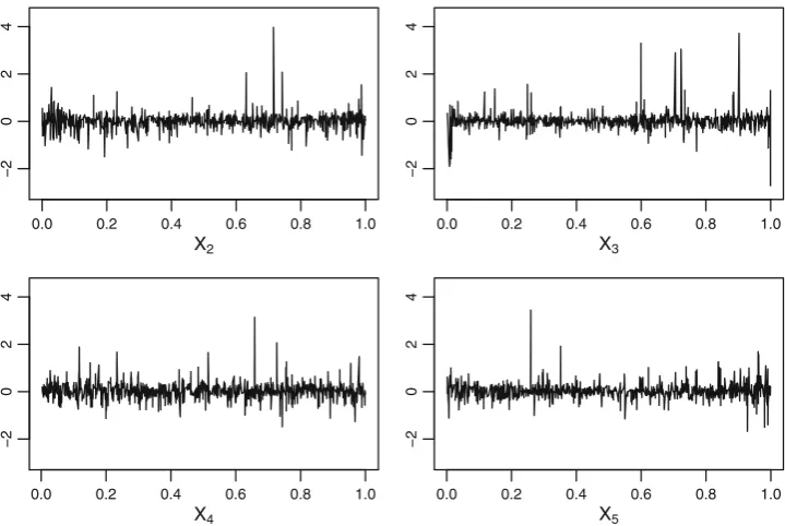
1000 conditional copulas, we calculate the log-likelihood deviation: the true log-likelihood subtracting the estimated log-likelihood. The four sequences of log-likelihood devia-tions are plotted in Fig.7.
For example, the top-left panel shows the evolution of the log-likelihood deviation for edge {1,3|2}, when the value of X2 increases from 0 to 1. Figure 7 shows that the true
likelihood is generally larger than the estimated log-likelihood, and the log-likelihood deviation fluctuates within a small range around zero.
From Remark2, we know that Eq. (6) can be used to test the simplifying assumption. As here we know the underlying true law, to examine the performance of the two-stage pro-cedure, we can also compare the true expected valueα(xe)
with its estimateαˆ(xe, μ∗):
ˆ
α(xe, μ∗)=
1
0
1
0
ˆ
ce˙1e˙2|De(u, w|XXXe =xe; μ∗)
h(u, w)dudw,
Fig. 7 Evolving paths of the difference between the true log-likelihood and the estimated log-likelihood (treeT2)
0.0 0.2 0.4 0.6 0.8 1.0
−2
0
2
4
X2
0.0 0.2 0.4 0.6 0.8 1.0
−2
0
2
4
X3
0.0 0.2 0.4 0.6 0.8 1.0
−2
0
2
4
X4
0.0 0.2 0.4 0.6 0.8 1.0
−2
0
2
4
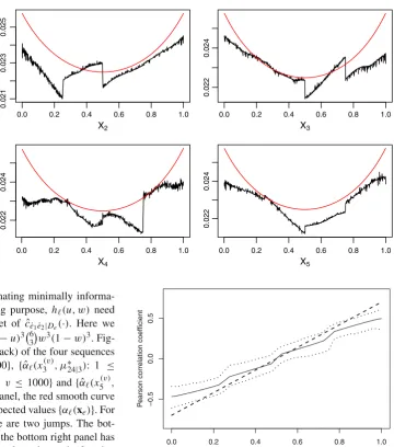
[image:13.595.54.289.52.213.2] [image:13.595.184.544.472.713.2]Fig. 8 Evolving paths of the true expected values{α(xe)}
(red) and of the estimated expected values{ ˆα(xe, μ∗)}
(black). (Color figure online)
0.0 0.2 0.4 0.6 0.8 1.0
0.021
0.023
0.025
X2
0.0 0.2 0.4 0.6 0.8 1.0
0.022
0.024
X3
0.0 0.2 0.4 0.6 0.8 1.0
0.022
0.024
X4
0.0 0.2 0.4 0.6 0.8 1.0
0.022
0.024
X5
wherecˆe˙1e˙2|De(·)is the approximating minimally informa-tive copula. Note that, for testing purpose, h(u, w) need not belong to the information set of cˆe˙1e˙2|De(·). Here we
might seth(u, w)to be63u3(1−u)363w3(1−w)3. Fig-ure8plots the evolving paths (black) of the four sequences
{ ˆα(x2(v), μ13∗|2): 1 ≤ v ≤ 1000}, { ˆα(x3(v), μ∗24|3): 1 ≤
v ≤ 1000},{ ˆα(x4(v), μ∗35|4):1 ≤ v ≤ 1000}and{ ˆα(x5(v), μ∗
46|5):1≤v≤1000}. In each panel, the red smooth curve
is the evolving path of the true expected values{α(xe)}. For
each of the top two panels, there are two jumps. The bot-tom left panel has one jump, and the botbot-tom right panel has two small jumps. The jumps in Fig.8are due to the fact that we assign different information sets to different subintervals. As we divide the[0,1]interval into four subintervals, there are at most three jumps. Yet, the four panels in Fig.8 all have jumps fewer than three, implying that the minimally informative copula evolves slowly even when the value of the conditioning variable crosses a splitting point. Figure8
shows that the estimated expected values are close to the true expected values; the relative errors are all within the interval (−0.02,0.08). Figures7and8(and figures in the supplemen-tary material) show that the two-stage procedure is capable of approximating conditional copulas.
We reuse the previously simulated 100 sets of data points (each with size 1000). For each data set, we have approximated the five bivariate copulas in treeT1; we now
approximate the conditional copulas in treeT2. Note that, for
each edge in treeT2, the conditioning variable always
dis-tributes uniformly in the[0,1]interval. Hence, it suffices to study only one edge, say edge{1,3|2}. For each value ofX2,
we first calculate the correlation coefficient of the true condi-tional copula and then numerically calculate the correlation
0.0 0.2 0.4 0.6 0.8 1.0
−0.5
0.0
0.5
X2
P
e
arson correlation coefficient
Fig. 9 The true and estimated correlation coefficients, varying with the value of the conditioning variableX2. The true correlation coefficient is shown as adashed curve, the average of the estimates taken over 100 Monte Carlo samples is displayed by the solid curve and the 90% Monte Carlo confidence intervals are given bydotted curves
coefficient of the approximating minimally informative cop-ula that is obtained from one data set. Since we have 100 data sets, we will have 100 such minimally informative copulas. In other words, for each value of X2, we will have one true
correlation coefficient and 100 estimating correlation coeffi-cients. We draw the 90% point-wise confidence intervals at 41 equally spaced grid points from 0 to 1; see Fig.9.
In Fig.9, it is observed that whenX2varies in, say, interval
(0.2, 0.8), the estimated correlation coefficient is close to the true correlation coefficient. However, when X2 is too large
or too small, the estimated correlation coefficient is biased. This is because the locally weighted average becomes biased approaching the boundary of the domain of X2, due to the
[image:14.595.184.545.48.457.2]