Time dependent road network design frameworks with land use consideration: policy implications

Word count: 6437+ 4*250=7437 words equivalent

TIME-DEPENDENT ROAD NETWORK DESIGN FRAMEWORKS WITH

LAND USE CONSIDERATION: POLICY IMPLICATIONS

Wai Yuen Szeto

Department of Civil Engineering National University of Singapore 1 Engineering Drive 2, E1A 07-03

Singapore 117576 Telephone: +65 65162279

Fax: +65-67791635 E-mail: [email protected]

Xiaoqing Li

Centre for Transport Research and Innovation for People (TRIP) Department of Civil, Structural and Environmental Engineering

Trinity College Dublin Dublin 2, Ireland Telephone: +353 1 896 2537

Fax: +353 1 677 3072 E-mail: [email protected] Margaret O'Mahony*

Centre for Transport Research and Innovation for People (TRIP) Department of Civil, Structural and Environmental Engineering

Trinity College Dublin Dublin 2, Ireland Telephone: +353 1 896 2084

Fax: +353-1-677-3072 E-mail: [email protected]

Submission date: 30th July, 2007

ABSTRACT

INTRODUCTION

Nowadays, many road network improvement projects are still ongoing, especially in some major cities in Asia and Europe. These projects are expensive. With respect to constrained government expenditure, especially for road network improvements, the government should carefully select cost-effective improvement projects to be implemented. Traditionally, the analysis involved belongs to the discipline of road network design. In the past, much research (e.g. 1-4) was

performed on the static approach to the discipline. Yang and Bell (5) provides a comprehensive

review on the static approach to this discipline. Recently, researchers consider the time dimension of transport network design. Three time scales are typically considered in the literature: seconds, days, and years. The smallest time scale (6) is used to capture the within-day

dynamics such as queuing phenomena, the fluctuation of demand within a day, and the departure choice of travellers. The medium scale (7) is used to capture the route adjustment behaviour of

travellers from day to day. The largest scale (8) is used to capture the changing demand, gradual

network upgrades, and cost and benefit over a long period of time, to maintain a similar social equity level over years, and to determine the optimal infrastructure improvement timetable, and its associated financial arrangement and tolling scheme.

All the previous efforts on transport network design, however, focus on the transport system alone and ignore the interaction between land use and transport over time. In reality, the transport system interacts with the land use system. When a new road is built or an existing road is widened, the travel costs between some zones decrease, and hence the accessibilities for those zones increase. Increases in the accessibilities lead to changes in population and employment distributions, and in turn a new travel demand pattern. The new travel demand pattern leads to a new traffic pattern and new congestion locations, which may require further improvements in the future. Ignoring the interaction may result in wrong allocations of budgets on (road) network improvements or starting the improvements at wrong locations or at a suboptimal time. In addition, the impact of road network improvement policies on the land use system, especially the benefit of landowners cannot be evaluated without considering the interaction.

In this paper, we develop a general time-dependent road network design framework encapsulating the Lowry-type land use consideration so that the land use transport interaction can be dealt with when determining optimal designs. More importantly, unlike existing models, the optimal designs can be determined automatically through the optimization procedure without trial-and-error once the objective is clearly defined. In addition, the effects of road network improvement policies on the land use side such as subsidizing road network improvements using public fund or transit revenue, cost recovery, and build-operate–transfer (BOT) on the profits of landowners and their profit distribution as well as population and employment changes can be studied using the proposed framework. The time scale we consider in the framework is in years as in Szeto and Lo (8), since the pace of the adjustment process inside the land use system is

found in this framework. The framework is formulated as a single-level single-objective optimisation program that can be solved by many existing optimization software.

To incorporate the considerations of various parties involved in road network improvement projects, a multi-objective optimisation framework is then developed through the hybrid approach. A numerical study using a small network is also set up to clearly illustrate the frameworks, the effect of the implementation of road network improvement projects on the related parties, and the tradeoffs between various objectives of the related parties, although the models herein can be used to handle general networks and eliminate many alternative designs. Three improvement schemes are considered: exact cost recovery, build-operate–transfer (BOT), and to use the increase in transit profit to subsidize road improvement projects. The scenario under each scheme is formulated individually using the proposed frameworks, and the corresponding optimal design is obtained by employing the generalized reduced gradient method (9) to solve the models. The results show that the changes in landowner profits are not the same

after implementing any one of three projects. This raises the issue of landowner equity in terms of changes in landowner profits. More importantly, the changes can be negative after the implementation. If we force the changes in landowner profits to be non-negative, societal benefit can be reduced and the road network can be more congested compared with the situation without enforcing non-negative changes in landowner profits.

The rest of the paper is organized as follows: The next section describes the formulation of the single-objective framework. The numerical study comes after that followed by the framework extension, the concluding remarks, the acknowledgement, and the references.

FORMULATIONS

We consider a strongly connected multi-modal transportation network with multiple Origin-Destination (OD) flows over the planning horizon

[ ]

0,T . The planning horizon is divided into

N equal design periods. The network is further divided into M subnetworks, one for each mode,

to account for the unique travelling speed of each mode. The mode here can be an individual mode or a combined mode. With this consideration, we can formulate the proposed framework as a single-level, single-objective constrained optimisation program as follows:

max ( )y x , (1)

subject to time-dependent Lowry-type constraints and modal-split/assignment constraints; road network design constraints;

financial constraints, and;

where y

( )

x is the objective function and x is the vector of decision variables including tolls and capacity enhancements. In the following, we discuss the framework.

Time-dependent Lowry-type Constraints and Modal-split/assignment Constraints

The time-dependent Lowry-type constraints are developed based on the Lowry-type land use model (10) and describe the interaction between employment and population over time according

(11) route choice behaviour in each design period based on the travel demand obtained from the

Lowry model. Due to space limitation, the details of the time-dependent constraints are not provided here. They can be found in Li et al. (12). Note that one of the differences between the

proposed single objective framework and the one in Li et al is that the latter is only consider time-dependent tolls while the former considers both time-dependent toll and capacity enhancement.

Road Network Design Constraints

They include link improvement constraints and toll constraints. Link improvement constraints are included to address the fact that a link (in road networks) cannot be built or expanded beyond an upper limit due to space limitation, and that the improvement must be non-negative. Toll constraints cater for scenarios that due to political reasons, the toll cannot be collected on certain links or set too high. These constraints can also be found in Li et al. (12).

Financial Constraints

They depict the relationship between the improvement costs, toll revenues, and subsidies. These constraints include cost and revenue functions and the cost recovery constraint.

Cost and revenue functions

The toll revenue T_τ , and the improvement and maintenance cost K_τ in period τ can be

expressed in terms of the equilibrium link flow m_, a

v _τ, the toll ρ_am_,τ and the improvement y_b,τ as

follows:

, , ,

m m a a m a

T_τ =

∑∑

nv _τρ _τ ∀τ, (2)

(

b, b,

)

, b

K_τ =

∑

h _τ +w _τ ∀τ , (3)

(

)

1

( )

,1

, 1 ,0 , , ,

b

b

b b b b

h _τ = + j% τ− b l y _τ ∀bτ , (4)

(

)

(

)

,2

1

, 1 ,0 ,1 , , ,

b

m

b b b b

m

w j nv b

β τ

τ β β τ τ

− ⎡ ⎛ ⎞ ⎤

= + ⎢ + _{⎜ ⎟} ⎥ ∀

⎝ ⎠

⎢ ⎥

⎣

∑

⎦

% , (5)

where h_b,τ and w_b,τ are the improvement (or construction) and maintenance cost functions of

link b in period τ respectively; b_b,0,b_b,1, β_b,0,β β_b,1, _b,2 are parameters of these cost functions; n converts link flows from an hourly basis to a period basis; %j is the inflation rate; l_b is the length

of link b. Equation (2) calculates the toll revenue in period τ , which is the sum of the product of the link flow and toll in that period. Equation (3) computes the improvement and maintenance cost in period τ by adding the improvement and maintenance cost of all links. Equation (4) is the time-dependent improvement cost function. The term

(

1+ j%

)

τ−1 represents the inflation factor:

for the same capacity enhancement, the improvement cost increases by j%% each period. The

term ,1

,0 ,1

b

b b b b

Equation (4) depicts the general relationship that the improvement cost of a link is proportional to the extent of the widening (and hence capacity gain,y_b,1) and its length. This function is

adopted for illustration and simplicity; other functional forms can be adopted in this framework without difficulty. Equation (5) is the time-dependent maintenance cost function, which is set to

be:

( )

,2

,0 ,1 ,1

b

m

b b b

m nv

β

β +β ⎛_⎜ ⎞_⎟

⎝

∑

⎠ in the base period, consisting of the fixed cost βb,0 and the variable

cost

(

)

,2 ,1 , b m b b m nv β τ

β ⎛_⎜ ⎞_⎟

⎝

∑

⎠ , in which

(

,

)

m b m

nv _τ

∑

is the link flow on link b in period τ . Again, the

maintenance cost depends on the inflation factor

(

1+ %j

)

τ −1.

Cost Recovery Constraints

Cost recovery can be classified into three types: partial, exact, and profitable (13). Partial (exact)

cost recovery occurs when the cost in a design period is partially (exactly) recovered by the revenue, adjusted to present value terms. Profitable cost recovery occurs when, in present value terms, the revenue more than covers the cost, with a surplus or profit at the end of the planning horizon. These three cost recovery schemes can be mathematically formulated using one equation:

( )

1

( )

1

( )

1

1 1 1

T S K

TOP

i i i

τ τ τ

τ τ τ

τ − τ − τ −

+ − =

+ + +

∑

∑

∑

% % % , (6)

where T_τ, K_τ, and S_τ are, respectively, the toll revenue from, the improvement and maintenance

cost, and the subsidy or contribution for network improvements in period τ ; TOP is the profit or surplus of the toll road operator; i% is the discount rate.

The first term on the left hand side (LHS) of (6) is the total discounted toll revenue for the entire planning horizon. Similarly, the second (third) term is the total discounted government subsidy (the total discounted improvement and maintenance cost). The cost recovery equation (6) requires that, in present value terms, the total toll revenue plus the total subsidy minus the total improvement and maintenance cost equals the surplus or profit. Depending on the values of

S_τ and TOP, equation (6) reduces to a) the partial cost recovery equation if S_τ is positive and

TOP is zero; to b) the exact cost recovery equation if all S_τ and TOP are zero; or to c) the profitable cost recovery equation if all S_τ are zero and TOP is positive.

In case the subsidy S_τ is obtained from the increase in transit profit (which is

numerically the same as the increase in transit revenue when the operation and maintenance cost is fixed.) k

U_τ′

Δ , the subsidy can be calculated by:

, ,

k k after k before

S_τ = ΔU_τ′=U_τ′ −U_τ′ , (7)

where k k_{, ,} k_{, ,} , ,

p ij p ij ij p

U_τ′ =

∑∑

p ′ _τnf ′ _τ ∀τ k′, (8)

where k_{, ,} p ij

p ′ _τ and U_τk′ are respectively the fare and revenue of transit mode k′ on route p

Equation (8) states that the subsidy due to the revenue of transit mode k′ is the sum of the product of the fare, k_{, ,}

p ij

p ′ _τ and the corresponding passenger flow nf_{p ij}k_{, ,}′ _τ in the period considered.

The Objective Functions

The objective function adopted depends on who is the decision maker. In the case the improvement projects involve the private sector (i.e. The builder and operator are the private sector) like build-operate-transfer projects, the objective is usually profit-maximizing, and the objective function is TOP defined by (6).

In the case where the funding is wholly from the government who is in charge of a road network design, the decision maker is the government who usually considers a number of objectives from the viewpoint of society. The main one is societal benefit, or equivalently the change in societal benefit after implementing a transport policy like implementing a road construction project (because the societal benefit before the implementation is a constant that does not affect finding the optimal design during optimisation). This can be measured by the change in social surplus (ΔSS), which is the difference between the SS after and before the implementation, and is equal to the sum of the change in consumer surplus (CS), ΔCS, the change in land owner profit, ΔLOP, the change in toll revenue, ΔT , the change in transit

revenue, ΔU , minus the change in net tax revenue, ΔR , the change in improvement and

maintenance cost for the toll road, ΔK, and the change in operation and maintenance cost of

transit modes, ΔY:

SS CS LOP T U R K Y

Δ = Δ + Δ + Δ + Δ − Δ − Δ − Δ . (9)

The change in consumer surplus, ΔCS, in equation (9) measures the difference between what consumers would be willing to pay for travel and what they actually pay. It internalizes the effect of network congestion and the public’s propensity to travel. For the same network and demand characteristics, a higher CS (positive change in CS) implies a better performing system.

The change in landowner profit ΔLOP is the sum of the change of each individual discounted land owner profit ΔLOP_j,τ over time:

(

)

, 1 1 j j LOP LOP i τ τ τ − Δ Δ = +

∑∑

. (10)

The difference of a land owner’ profit before and after the network improvement project implementations can be written as follows:

, , , , ,

after before

j j j

LOP_τ LOP_τ LOP_τ jτ

Δ = − ∀ , (11)

where , before j

LOP_τ and , after j

LOP_τ represent the profits of land owner j before and after the network

improvement project implementation in period τ .

The change in toll revenue ΔT can be similarly calculated by:

(

)

( )

1

1 after before T T T i τ τ τ τ − − Δ = +

∑

_% . (12)

The term in the numerator is the difference of toll revenue after and before the implementation of network improvement projects. This term is discounted by 1 ₁

change in toll revenue in period τ . The sum of the discounted change in toll revenue in all periods is the change in toll revenue according to (12).

The change in transit revenue can be defined in a way similar to the change in toll revenue:

(

)

( )

, , 1 1

k after k before

k U U U i τ τ τ τ ′ ′ − ′ − Δ = +

∑∑

_% . (13)

where k

U_τ′ follows the definition in (8).

The change in tax revenue, ΔR , is equal to the total discounted subsidy from the

government,

( )

1

1

S

i

τ τ

τ + −

∑

% . There is only one term in the numerator as the subsidy before the

implementation is zero.

Similarly, the change in improvement and maintenance cost for toll roads, ΔK, can be

defined like the change in tax revenue:

( )

1,

1 K K i τ τ τ − Δ = +

∑

_% (14)

Again, the improvement and maintenance cost is zero before the implementation, so there is only one term in the numerator.

The change in operation and maintenance cost of transit ΔY is actually zero if we assume

this cost is fixed and independent of the number of passengers.

Considerations in Road Network Improvement Projects

Developing a specific model requires taking into account the parties involved in the implementation of road network projects. In general, the implementations of road network projects involve many parties, including road users, private landowners, private transit operators, private toll road operators, and the government. Each of these parties has distinctive objectives as discussed below.

Road users: the shortest travel time and the lowest travel cost

Travellers are concerned with their actual travel times and travel costs. The actual travel time is the shortest travel time between an OD pair. The travel cost is the sum of the travel time cost and the toll required to pay in which the travel time cost is the product of the value of time and the shortest travel time.

Private Landowners: Discounted Profit or the Change in Landowner’s (Discounted) Profit

In the case of private landowners, they are concerned with their own total discounted profit, which is the sum of the discounted landowner profit in each year. This can be formulated as:

( )

, 1, 1 j j LOP LOP j i τ τ τ − = ∀ +

where LOP_j is the discounted profit of landowner j. After the project implementation, there

must be a change in landowner profit due to redistribution of residents. This change in landowner’s profit can be used as an alternative to formulate the objective of the landowner, since the profit before the implementation is fixed. This change can be written as:

( )

,1, 1 j j LOP LOP j i τ τ τ − Δ

Δ = ∀

+

∑

_% , (16)

where ΔLOP_j,τ is defined in equation (11). A positive value of ΔLOP_j means the project

implementation is beneficial to the landowner, and vice versa.

Private Transit Operators: Profit

Like private landowners, the objectives of transit operators are profit-driven. The profit of the private transit operator can be written as:

( )

1,

1 k k k U Y U k i τ τ τ τ ′ ′ ′ − − _′ = ∀ +

∑

% , (17)

where k

U_τ′ is the revenue of transit operator k′ in period τ defined in (8); Y_τk′ is the operation

and maintenance cost of transit operator k′ in period τ .

Private Toll Road Operators: Profit

The objective of each private toll road operator is to maximize his/her total discounted profit b

TOP, which is the difference between the total discounted revenue T_b and the total discounted

cost K_b:

, b b b

TOP = −T K ∀b, (18)

where

( )

, ,1, 1 m m a a b m nv T b i τ τ τ τ ρ − = ∀ +

∑∑

_% ; (19)

( )

, 1, 1 b b h K b i τ τ τ − = ∀ +

∑

% ; (20)

The subscript b represents the toll road operator; nvam_,τρam_,τ is the toll revenue in period τ from mode m on road networks, and h_b,τis the improvement cost.

Government: Average Network Travel Time, Equity between Landowners

The government has a lot of concerns, including the whole societal benefit, the congestion problem, the environmental issue, the equity issues between travellers, between private toll road operators, and between landowners, and so on. Here we only discuss two measures: the average network travel time, and the equity constraints between landowners.

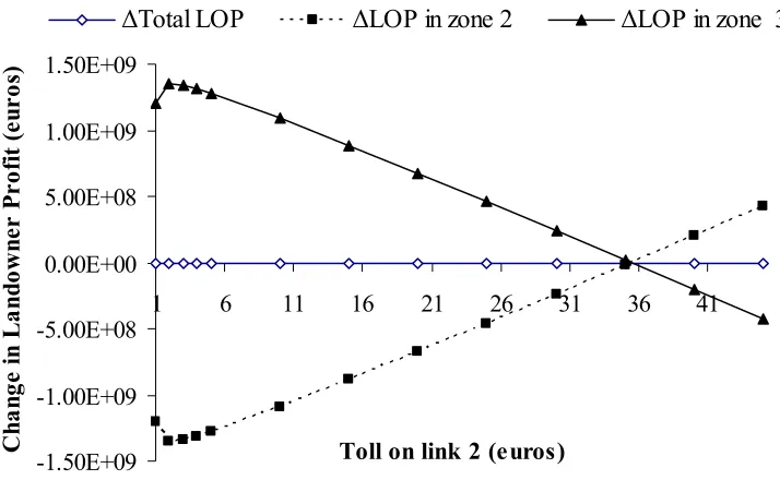
In general, the implementation of road improvement projects may result in different changes in landowner profits. Some changes can be greater than others, and some changes can be even negatives. This raises the issue of equity between landowners. Here we consider that in the simplest case of equity: all changes must be nonnegative. If all changes are nonnegative, we say that inequity does not exist.

Three Models Derived from the Proposed Single-objective Framework

Based on the considerations above as well as different combinations of objective functions and constraints discussed above, we can develop many specific single-objective optimisation models. In this section, three specific models are provided, which will be used in the numerical study. They are the profit maximization model, the social surplus maximization model under exact cost recovery, and the social surplus maximization model under cross-subsidization:

Profit Maximization Model (PM model)

The profit maximization model can be obtained by setting y

( )

x in (1) to be TOP defined by (6):

max TOP

E,R,f,y,ρ

subject to time-dependent Lowry-type constraints and modal-split/assignment constraints; road network design constraints, and;

financial constraints (2)-(5),

where E, R,f, y,ρ represent, respectively, the vectors of the number of service employment trips, the number of work-to-home trips, path flows, capacity improvement, and tolls. Note that the cost recovery condition (6) is included in the objective function rather than in financial constraints. This model is suitable to aid decision-making in the build-operate-transfer projects.

Cost Recovery Model (CR model)

This can be formulated as follows: max SSΔ

E,R,f,y,ρ

subject to the same constraints as in the PM model, and;

the cost recovery condition (6) with TOP=0 and S_τ = ∀0, τ,

where ΔSS is defined by (9). This model formulates the problem from the government’s perspective, assuming the toll revenue generated to be able to recover the improvement and maintenance cost. In the case when the improvement and maintenance cost is very expensive and the toll revenue generated is not able to recover the cost, the model gives no improvement, zero toll charges and no change in SS.

Cross-subsidization Model (CS model)

This can be formulated as follows: max SSΔ

E,R,f,y,p

where p is the vector of transit fares. This model also formulates the problem from the perspective of the government, assuming that there is a transit profit and the increase in profit is enough to build the toll road. In reality, the change in transit profit can be negative but the transit can still have a profit. In this case, the profit can still be used to subsidize the toll road construction and its maintenance but the cross-subsidization condition requires modifications.

Model Extension: Multi-objective Optimisation Multi-optimisation Framework

The above single-objective optimisation model may not be able to give a design that makes every party happy, as will be shown in the numerical study. If this happens, we find a compromised design using the following multi-objective optimisation framework extended from the proposed framework discussed before:

max _{i i}( )

i

w y

∑

x , (21)

subject to the same as the single-objective framework; 1

i i

w =

∑

; (22)

0

i

w ≥ ; (23)

( )

j

y% x ≥ε; (24)

where yi

( )

x is the i-th (normalized) objective function; x is the vector of decision variables; i

w is the (normalized) weight for i-th objective function; ε is the aspiration level or the

satisfactory objective value, and y%j

( )

x is the j-th objective function that does not appear in the weighted objective function in (21).

In the above framework, objective function (21) is formed by summing all the weighted objective functions. Condition (22) is the weight constraint, which requires the sum of all weights to be one to normalize all the weights. Condition (23) is the nonnegativity condition of the weights. Condition (24) is the performance constraint (or ε - constraint), which considers the objective that does not include in (21). The objective function is set to be greater than the desirable or satisfactory objective value to ensure that at optimal, but the j-th objective value is

at least equal to the satisfactory value.

Two points are worth mentioning. First, the weights are input, and their relative magnitudes represent the relative importance of those objectives. Second, the larger the value of

ε, the tighter the constraint and the closer to the optimal j-th objective value at optimal. The

following is an example of the performance constraint.

Equity Constraints

The landowner equity constraints can be expressed as: 0,

j

LOP j

Δ ≥ ∀ , (25)

Cost Recovery Model under Equity Consideration (CR-equity model)

This multi-objective optimisation model will be used in the numerical study and is formulated as follows:

max SSΔ

E,R,f,y,ρ

subject to the same constraints as in the CR model, and; the landowner equity constraint (25)

where ΔSS is defined by (9). The key difference between this model and the CR model is that this model has the landowner equity constraints, avoiding reduction in landowner profit due to the implementation of network improvement projects.

NUMERICAL STUDY

This study is set up to compare the three schemes of road network design, namely build-operate-transfer, cost recovery, and cross subsidization, illustrate the impacts of the implementation of road network improvements on the related parties, especially on landowners, and show the tradeoffs between various objectives of the related parties. The build-operate-transfer (BOT) scheme allows a private company to build a toll road and collect tolls to recover the construction and maintenance cost within a franchised period; and after the franchised period is over, all these toll roads are transferred back to the government. This scheme is very common now in Asia and Europe. The exact cost recovery scheme uses toll revenue to exactly recover the construction and

[image:12.612.142.497.487.617.2]

maintenance cost. The tolling and improvement strategy is to maximize the change in SS, rather than to maximize the profit as in the BOT scheme. Since the objective of this scheme is to maximize the change in SS, the private sector is not willing to be involved. The builder and operator is thus the government. This scheme can be found in India. The cross subsidization scheme is similar to the exact cost recovery scheme except that the increase in transit profit is used to subsidize the construction and maintenance cost of the toll road. This scheme is not common and only applicable to the place like Ireland whether the transit system is government-owned and can generate a huge profit.

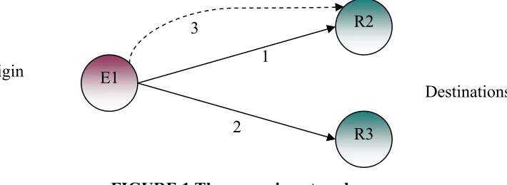
FIGURE 1 The scenario network.

Scenario Setting

For the ease of exposition, a simple network is adopted as shown in figure 1. There are 3 links in this network: link 1, link 2, and link 3. Links 1 and 2 are links whose travel time is given by the BPR functions. Link 3 is a separate transit link, as represented by a dash line in the figure. There are 3 zones too: E1, R2, and R3, in which ‘E’ stands for an employment zone whereas ‘R’ stands

E1

R3 R2

2 1 Origin

3

for a residential zone. The attractiveness of each zone is assumed to follow the following function:

(

)

, 1 , 1 ,

i i w i

Wα_τ+ =Wα_τ +h% ,

where h%_{w i,} is the growth rate of attractiveness of zone i over time. The basic employment in the

employment zone is supposed to grow linearly over time:

(

)

, 1 , 1 ,

B B

i i E i

E _τ+ =E_τ +h% ,

where h%_{E i,} is the growth rate of basic employment. The three zones form two OD pairs: E1-R2

and E1-R3. Both OD pairs are connected by highways but only OD pair E1-R2 has a separate transit connection. In other words, there are two modes for OD pair E1-R2 but there is only one mode for OD pair E1-R3.

The parameters in this study include: a) Land use parameters:

1,1 B

E =5000 jobs; W_1,1α =3000 jobs; W_2,1α =W_3,1α =3000 houses; population to employment ratio,μ =5; service employment to population ratio,s=0.1; parameter to regulate the effect of travel cost on distribution of residents,βr =_0.04€ -1_{; parameter to regulate the} effect of travel cost on distribution of service employment, βs = _{0.03 €} -1_{; fixed} maintenance cost on houses in residential zones j in period τ , M%_j,τ = €100; maintenance cost per house, h €0.01

m = /household; h%_w,1=h%_w,2 =h% = 0.05; _w,3 h_E,1 =0.04,

rent per house in residential zone j in period τ , r_2,0=r_3,0 =12 ×€1000 × 10 = €120000

b) Transport network parameters: Initial capacity, 0 0

1 2

c =c =3000 vph; capacity upper bound, u₁ =u₂ = 10000 vph; free

flow travel time, 0 0

1 2

t = =t 5 hours; t₃0 =4 hours

c) Transit’s operation and maintenance cost in period τ : 2

Y_τ =1000000 €

d) Parameters of improvement cost functions: b_1,1=b_2,1=1, b_1,0 =b_2,0=€ 2000

e) Parameters of maintenance cost functions: β_2,0= €1200, β_2,1= €0.001, β_2,2=1

f) Parameters in travel cost functions: Value of time, ψ = €15/h; mode-specific cost, car

θ =16; θtransit =_{30; parameter to regulate thecomposite cost,} β =_0.05€ -1 g) Interest and inflation rates: i%=0.03; %j=0.01

h) Converting factor: n=365days×24hours ×10 years = 87600hours/period i) Length of each period: 10 years

j) Planning horizon and franchised period:

[

0,50

]

. k) Specific parameters for each scheme:

a. BOT: the transit fare on link 3 between OD pair E1-R2 in period τ , 2 3,12,

p _τ =€40; the toll on link 1,ρ1,τ =€0; Maximum allowable toll: ρmax= € 5

b. Cost recovery: the transit fare on link 3, 2 3,12,

c. Cross-subsidization: the tolls on both links 1 and 2,ρ_1,τ = ρ_2,τ =€0; These values are chosen for illustrative purposes.

Performance of Each Scheme

The optimal designs under the three schemes are obtained by solving the PM model, the CR model, and the CS model using the generalized reduced gradient method (9). The corresponding

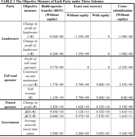
performance measures are shown in table 1 and figure 2. In general, they show that road network improvements have different impacts on related parties, including road users, private landowners,

[image:14.612.69.543.231.711.2]

transit operators, private toll road operators and, the government.

TABLE 1 The Objective Measure of Each Party under Three Schemes Exact cost recovery Party Objective

measure

Build-operate-transfer (BOT)

(Without

equity) Without equity With equity

Cross-subsidization

(Without equity) Change in

profit of landowner

2 (€) -9.26E+08 -1.35E+09 0 -1.94E+08

Landowners

Change in profit of landowner

3 (€) 9.26E+08 1.35E+09 0 1.94E+08

Profit of toll road

operator 9.77E+09 0 0 -2.55E+09

Constructi on and maintenan

ce cost (€) 1.77E+09 5.79E+09 5.80E+10 2.55E+09

Toll road operator

Toll revenue

(€) 1.15E+10 5.79E+09 5.80E+10 0.0E+00

Transit operator

Change in

profit (€) 2.43E+10 1.62E+10 4.53E+10 2.55E+09

ΔSS (€) 9.45E+10 1.12E+11 4.52E+10 1.61E+11

ΔCS (€) 6.04E+10 9.57E+10 -7.87E+07 1.61E+11

Government Average

network travel time

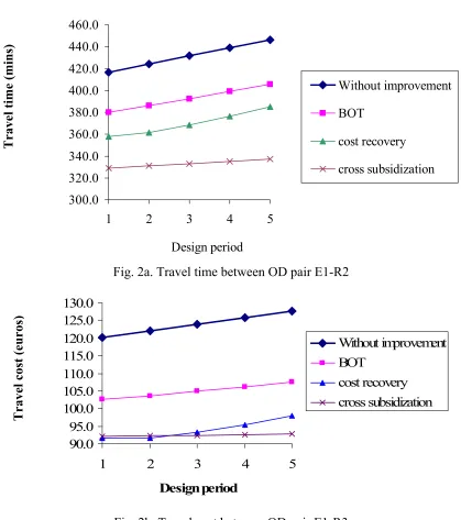
300.0 320.0 340.0 360.0 380.0 400.0 420.0 440.0 460.0

1 2 3 4 5

Design period

Without improvement

BOT

cost recovery

[image:15.612.96.515.86.559.2]

cross subsidization

Fig. 2a. Travel time between OD pair E1-R2

90.0 95.0 100.0 105.0 110.0 115.0 120.0 125.0 130.0

1 2 3 4 5

Design period

Without improvement BOT

cost recovery cross subsidization

[image:15.612.158.366.99.319.2]

Fig. 2b. Travel cost between OD pair E1-R3

FIGURE 2 Travel time and travel cost over time.

Road Users

They are concerned with their travel times and travel costs. According to Figure 2, the travel times and travel costs increase over time due to increase in population over time and increase in travel demand. However, after the implementation of any road improvement projects, travel time and travel cost are less than those before.

Travel time

(mins

)

Travel cost

(euros

[image:15.612.152.503.356.539.2]

Private Landowners

Private landowners are concerned with their own profit. As shown in table 1, without considering the equity of land owners, the profit of landowner 2 will be reduced but that of landowner 3 will be increased if any one of the schemes is implemented. Landowner 2 will object to any implementation unless the government provides him/her a subsidy to raise the profit back to the original level.

Toll Road Operators

Private toll road operators are concerned with the profit from the project. Without considering the equity of land owners, the BOT scheme will result in generating a profit, but this profit may not be too attractive as the rate of return (i.e. toll revenue/construction and maintenance cost) is about 6%, which is less than the usual norm of 10-15 %. From the private toll road operator viewpoint, the project is not attractive if no subsidy is further given from the government. However, if the government gives the operator a subsidy to raise the rate of return to the minimum of 10%, the SS will decrease further.

It is worthwhile to point out that in the cost recovery scheme, the builder and operator is the government, whose objective is to maximize the change in SS subject to cost recovery. So you can see in table 1 that the profit is zero and the construction cost and maintenance cost is equal to the toll revenue.

Transit Operators

When the transit operator is private and profit-driven, without considering the equity of land owners the operator will welcome the implementation of the BOT and the cost recovery scheme because both schemes will raise the higher transit profit, in particular the operator will prefer the BOT scheme more as the change is larger.

When the transit operator is the government, the positive change in transit profit means the implementation is good to society, as the change in transit profit (or the change in transit revenue minus the change in transit’s operation and maintenance cost) is part of the change in SS. Note that under cross-subsidization, the change in transit profit is equal to the construction and maintenance cost of toll roads.

Government

From the government’s perspectives, the three schemes are beneficial to society, as the change in social surplus (ΔSS) is positive. In addition, from the congestion or road network performance point of view, the three schemes do improve the situation, since the change in consumer (ΔCS) is positive and the average network travel time is lower than 437 minutes which is the average network travel time without the implementation of any scheme. However, the government needs to consider the unequal change in profit between the landowners when any one of these schemes is implemented and may require subsidizing the private toll road operator when the BOT scheme is implemented.

the government point of view. The BOT scheme gives the largest profit from toll and transit revenue, and is the best from the private transit and toll road operator point of view. When the transit operator is private, cross-subsidization is not possible and exact cost recovery gives a better performance in terms of ΔSS, ΔCS, and the average network travel time. Then, cost recovery is the second best. However, all these observations and conclusions are based on this specific case, and cannot be generalized to another study. Nevertheless, a general observation can be made. All schemes can lead to an unequal change in landowner profit, and some landowner’s profit can be reduced. Landowners will object to the implementation of the scheme

if this happens. To avoid this happening, we have to take their consideration into account when designing road improvement projects.

Performance of the Cost Recovery Design under Landowner Equity Consideration

To deal with the consideration of landowners, we can add equity constraints to the three models, ensuring that the changes in landowner profits are nonnegative. For illustrative purposes, we only add equity constraints to the CR model to form the CR-equity model. This CR-equity model is solved by the generalized reduced gradient method, and the performance measures with and without landowner equity considerations are also provided in table 1.

These results clearly show tradeoffs between the perspectives of each of the parties. The

equity scheme is worse than the original cost recovery design in terms of ΔSS, ΔCS and the average network travel time. ΔSS and ΔCS are smaller and the average network travel time is higher, meaning that society receives less benefit and the road network is more congested when we ensure landowner equity. In particular, ΔCS is negative, which is highly unacceptable. Road travellers face higher travel time and cost compared with the situation without considering equity. However, the private transit operator will favour the equity scheme as the change in profit is larger.

[image:18.612.150.507.85.305.2]

FIGURE 3 Changes in landowner profits against toll on link 2.

CONCLUSIONS

This paper proposes a single-objective road network design framework for considering the land-use transport interaction over time. This framework allows the evaluation of the impact of the design on related parties including landowners and contrasts to existing models that cannot be used for such purpose as the land use transport interaction over time is not captured. This flexibility helps network planners and private firms with decision-making. This framework is formulated as a single-level maximization program, and can be solved by many existing optimisation methods. Through the hybrid approach, the framework is also extended to consider multi-objectives. This multi-objective framework can aid the government making decisions considering the objective of each related party and eliminating a large number of alternative designs without trial-and-error.

This paper also illustrates the models and the impacts of road network improvements on related parties, especially landowners, under different network design schemes through a simple example, although the models can be applied to general networks. The results show that it is difficult to comment which scheme is the best in general after considering each party’s perspective and that tradeoffs exist between the objectives of all related parties. Moreover, all schemes lead to unequal changes in landowner profits. This raises the issue of landowner equity. If we aim at ensuring that their profits must not be reduced, other considerations such as societal benefit and the road network performance may get worse. Therefore, the government has to carefully consider the tradeoffs.

This paper opens up a number of research directions. First, the proposed frameworks only consider single class drivers with one trip purpose and the Wardrop’s travel principle. A possible

-1.50E+09 -1.00E+09 -5.00E+08 0.00E+00 5.00E+08 1.00E+09 1.50E+09

1 6 11 16 21 26 31 36 41

Toll on link 2 (euros)

C

han

ge

in

L

an

do

w

ne

r P

rof

it

(

eu

ros

)

direction is to extend them to consider multi-class drivers in which each class of driver has its own value of time, routing strategy, and trip purpose. Second, the network and the demand here are assumed to be deterministic. In reality, they are not. Capturing uncertainty in demand and supply in the proposed frameworks can be another direction. Third, BOT projects are in fact competing with others. It is thus worthwhile to extend the proposed framework to model the competitive situation between BOT projects.

A

CKNOWLEDGEMENT

This research is funded under the Programme for Research in Third-Level Institutions (PRTLI), administered by the Higher Education Authority.

REFERENCES

1. Davis, G. A. Exact Local Solution of the Continuous Network Design Problem via Stochastic User Equilibrium Assignment. Transportation Research, Vol. 28B, 1994. pp. 61-75.

2. Meng, Q., H. Yang, and M. G. H. Bell. An Equivalent Continuously Differentiable Model and A Locally Convergent Algorithm for the Continuous Network Design Problem.

Transportation Research, Vol. 35B, 2001, pp. 83-105.

3. Chen, A., and C. Yang. Stochastic Transportation Network Design Problem with Spatial Equity Constraint. In Transportation Research Record: Journal of the Transportation

Research Board, No. 1882, TRB, National Research Council, Washington, D.C., 2004, pp.

97–104.

4. Chiou, S. W. Bilevel Programming for the Continuous Transport Network Design Problem.

Transportation Research, Vol. 39B, 2005, pp. 361-383.

5. Yang, H., and M. G. H. Bell. Models and Algorithms for Road Network Design: A Review and Some New Developments. Transport Reviews, Vol. 18(3), 1998, pp. 257-278.

6. Heydecker, B. G. Dynamic Equilibrium Network Design. Transportation and Traffic Theory in the 21st Century. Pergamon Press, Oxford, pp. 349-370, 2002.

7. Friesz, T. L., and S. Shah. An Overview of Nontraditional Formulations of Static and Dynamic Equilibrium Network Design. Transportation Research, Vol.35B, 2001, pp. 5-21.

8. Szeto, W. Y., and H. K. Lo. Transportation Network Improvement and Tolling Strategies: The Issue of Intergeneration Equity. Transportation Research, Vol. 40A, 2006, 227-243.

9. Abadie, J., and J. Carpentier. ‘Generalization of the Wolfe Reduced Gradient Method to the Case of Nonlinear Constraints’, in R. Fletcher (ed.), Optimization, Academic Press, New

York, pp. 37-47, 1969.

10.Lowry, I. S. A Model of Metropolis. RM-4035- RC. Rand Corporation, Santa Monica, CA, U.S.A, 1964.

11.Wardrop, J. Some Theoretical Aspects of Road Traffic Research. Proceedings of the Institute of Civil Engineers, Part II, 1952, pp. 325-378.

12.Li, X. Q., W. Y. Szeto, and M. O’Mahony. Incorporating Land Use, Transport and Environmental Considerations into Time-dependent Tolling Strategies. Journal of the Eastern Asia Society for Transportation Studies, accepted, 2007.