Generalizing boundaries for triangular designs, and efficacy estimation at extended follow ups

M E T H O D O L O G Y

Open Access

Generalizing boundaries for triangular

designs, and efficacy estimation at extended

follow-ups

Annabel Allison

, Tansy Edwards

, Raymond Omollo

, Fabiana Alves

, Dominic Magirr

and Neal D. E. Alexander

Abstract

Background: Visceral leishmaniasis (VL) is a parasitic disease transmitted by sandflies and is fatal if left untreated. Phase II trials of new treatment regimens for VL are primarily carried out to evaluate safety and efficacy, while pharmacokinetic data are also important to inform future combination treatment regimens. The efficacy of VL treatments is evaluated at two time points,initial cure, when treatment is completed anddefinitive cure, commonly 6 months post end of treatment, to allow for slow response to treatment and detection of relapses.

This paper investigates a generalization of the triangular design to impose a minimum sample size for

pharmacokinetic or other analyses, and methods to estimate efficacy at extended follow-up accounting for the sequential design and changes in cure status during extended follow-up.

Methods: We provided R functions that generalize the triangular design to impose a minimum sample size before allowing stopping for efficacy. For estimation of efficacy at a second, extended, follow-up time, the performance of a shrinkage estimator (SHE), a probability tree estimator (PTE) and the maximum likelihood estimator (MLE) for estimation was assessed by simulation.

Results: The SHE and PTE are viable approaches to estimate an extended follow-up although the SHE performed better than the PTE: the bias and root mean square error were lower and coverage probabilities higher.

Conclusions: Generalization of the triangular design is simple to implement for adaptations to meet requirements for pharmacokinetic analyses. Using the simple MLE approach to estimate efficacy at extended follow-up will lead to biased results, generally over-estimating treatment success. The SHE is recommended in trials of two or more treatments. The PTE is an acceptable alternative for one-arm trials or where use of the SHE is not possible due to computational complexity.

Trial registration: NCT01067443, February 2010.

Keywords: Randomized trials, Sequential methods, Triangular boundaries, Visceral leishmaniasis, Shrinkage estimator

Background

Visceral leishmaniasis (VL) is a parasitic disease transmit-ted by sandflies and is fatal if left untreatransmit-ted. It is estimatransmit-ted that there are 0.2–0.4 million incident cases per year, with the six worst affected countries—India, Bangladesh, Sudan, South Sudan, Ethiopia and Brazil—reporting more than 90 % of them [1].

*Correspondence: [email protected] 1Lancaster University, LA1 4YW Lancaster, UK

2The University of Sheffield, Western Bank, S10 2TN Sheffield, UK Full list of author information is available at the end of the article

Until recently, the first-line treatment for VL was daily injections with the antimonial compound sodium sti-bogluconate for 30 days. The current first-line treat-ment in eastern Africa is 17 days of daily injectable doses of sodium stibogluconate and paramomycin [2]. Sodium stibogluconate is associated with cardiotoxicity, and drug resistance is a concern in Asia [3]. From a pub-lic health perspective, safe and efficacious short-course combination therapies of less than 2 weeks duration with one or two oral treatments would be considered most desirable [3].

A number of trial designs have been adopted in the con-duct of clinical trials against VL and other neglected trop-ical diseases, with the use of adaptive/sequential designs gaining prominence, particularly for Phase II trials. In par-ticular, the triangular design allows for repeated interim analyses, each on a relatively small number of patients, to efficiently triage between poorly performing treatments and those showing promise for further investigation (e.g., inclusion in a Phase III trial) [4]. Effectively, the design acts as a decision tool for whether or not a treatment merits continued study. By pre-specifying the power, Type I error, and null and alternative values for the outcome (e.g., proportion cured), a closed continuation region is drawn with upper and lower boundary lines forming a triangular shape. If higher values are beneficial, then crossing the upper boundary corresponds to stopping for promise, while crossing the lower boundary corresponds to stopping for lack of promise. Variations on the design accommodate comparative trials [5].

The estimation of efficacy at the end of the trial using the full sample of data needs to account for the multi-ple interim analyses, which lead to bias in the maximum likelihood estimator (MLE), e.g., the simple proportion of the number of patients cured divided by the number of treated. One suitable option is the median unbiased esti-mate (Chapter 5 in [6]), which can be found using software such as R or SAS.

In VL treatment trials, there are two important efficacy endpoints: initial cure and definitive cure. After comple-tion of treatment, initial cure status is established before the patient is discharged. In a clinical trial with a para-sitological assessment conducted as standard at the end of treatment, a patient may have:

• cleared parasites (initial treatment success) • parasites remaining but with clinical improvement,

so that additional treatment is not considered to be required prior to discharge (potential slow responder to treatment)

• parasites remaining and clinical improvement not shown, and so they require rescue treatment prior to discharge (confirmed treatment failure)

For those not needing rescue treatment, definitive cure is assessed after a period of time (usually 6 months post end of treatment) due to the possibility of (1) slow response to treatment and (2) relapse following an initial treatment success. Slow response to treat-ment is confirmed with an additional clinical and par-asitological assessment, usually 1 month after end of treatment. If parasites are cleared, the patient does not need rescue medication, this being a subset of treat-ment success at definitive cure. If parasites remain, the patient will have indication of rescue treatment, and

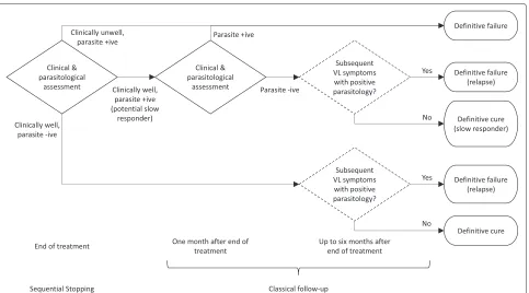
will be considered a definitive failure at the 6 months’ follow-up. Future research direction decisions are based on definitive cure at the end of the follow-up period, as patient status may change between end of treat-ment and final definitive assesstreat-ment. Figure 1 high-lights the different assessment time points and possible outcomes.

In a Phase II randomized trial of VL treatments in Sudan and Kenya, a triangular continuation region was defined for each of the three arms [7]. In this trial, the primary endpoint, used for sequential decision-making, was initial cure: a binary outcome defined by absence or presence of parasites at end of treatment. This endpoint permitted the prompt identification of poorly performing treatments. Use of definitive cure in sequential decision-making was deemed not to be feasible due to implications for time to trial completion and the potential to expose an unaccept-able number of patients to ineffective treatments.

The investigators found it necessary to modify the stan-dard triangular design in two ways. Firstly, a pharmacoki-netic (PK) evaluation component required a minimum of 30 patients, whereas the interim analysis was to be done after every 15 patients had completed the end-of-treatment assessment. So recruitment was to continue even if the upper boundary was crossed at the first interim analysis. Secondly, although standard sequential meth-ods sufficed for the end-of-trial analysis of initial cure, a new methodology was needed for point and interval estimation for definitive cure, to account for sequen-tial stopping, then non-sequensequen-tial follow-up, operating in tandem.

The first modification ignored the impact on Type I and II errors, rather than attempting to adjust the stan-dard continuation region. And the second modification consisted of a simple probability tree argument whose effi-ciency, in the statistical sense of low standard error, was not evaluated.

Aims

Hence, in the current paper, we aim to derive methods for the following two distinct aspects of such trials:

• definition of flexible boundaries that generalize simple triangular ones to prevent stopping before a given number of patients, while maintaining nominal error probabilities

• estimation, by shrinkage and other methods, of the outcome variable (e.g., cure) at a time point later than that used for the sequential stopping rule

Motivating example

Fig. 1Flowchart outlining the assessments in a visceral leishmaniasis trial. A diagram showing the different clinical and parasitological assessment time points carried out and possible outcomes in a VL trial

arm having the same triangular boundary and being sub-ject to the same stopping rules independently of the other two arms.

It was assumed that a day 28 cure rate ofp0 = 0.75 could be achieved on standard care. Denoting the day 28 cure rate on treatmentjbypj, the treatment effects were

parameterized as

θj=log

pj(1−p0) (1−pj)p0

, θj∈(−∞,∞), j=1, 2, 3. As a cure rate of 0.9 would be considered sufficiently promising to warrant further investigation, in this case

θR=log

0.9(1−0.75)

(1−0.9)0.75

=1.10.

The Type I and Type II error rates were both set at 5 %, so it was required that for each null hypothesisH0j:θj=0,

j=1, 2, 3:

P(rejectH0j;θj=0)=0.05, (1)

P(rejectH0j;θj=θR)=0.95. (2)

Omollo et al. found the boundaries using analytical results specific to a triangular test, as described by Ranque et al. [8], rather than numerical integration. From the planned frequency of interim analyses—every 15 patients in each arm—and other parameters such as the error probabilities, equations for the upper and lower straight line boundaries are obtained. The maximum sample size

is given by the intersection of these lines, in this case 63 per arm.

An additional complication in this trial was that at least 30 patients were required to assess PK. Therefore, although crossing the lower boundary at the first interim analysis would result in the arm being stopped for ethi-cal reasons, crossing the upper boundary was to be dis-regarded, with recruitment continuing until the second interim analysis. This partial disregarding of the bound-aries affects the stopping probabilities and hence, deviates the error probabilities from their nominal values. This was ignored in the trial described by Omollo et al., but such modified stopping rules are developed formally in the current paper, and we derive corresponding adjustments under asymmetric stopping or unequally spaced analyses.

Methods

The group-sequential triangular design

To review the triangular design briefly [6], consider a parameter of interest,θ, which could represent either the advantage of an experimental treatment over a control arm in a two-arm study, or relative to a fixed null value in a single-arm trial. The null hypothesis to be tested isH0: θ = 0 against the alternativeH1:θ > 0, subject to error constraints:

P(rejectH0;θ =0)=α (3)

for suitably smallαandβ, whereθRrepresents the small-est possible treatment effect size that would be considered interesting or clinically relevant.

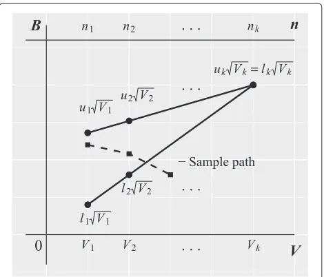
There areklooks at the data, with the data available at theith interim analysis summarized in terms of the effi-cient score forθ, denoted byBi, and Fisher’s information,

denoted byVi(see p. 107 [9]). For most types of data, there

is a straightforward relationship between Fisher’s infor-mation and the sample size,ni. For example, for a single

stream of binary dataVi=nip(1−p), wherepis the

suc-cess probability [6]. Two key assumptions underpinning most sequential methods are thatBi ∼ N(θVi,Vi), and

that (Bi+1−Bi) andBiare independent,i=1, 2,. . .. The

standardized test statistic is denoted byZi =Bi/√Viand

follows the standard normal distribution whenθ =0 [10]. These assumptions have been shown to be valid for a wide variety of response types [6].

The efficient score is compared to a set of upper and lower boundary values at theith analysis,i=1,. . .,k. At the first(k−1)interim analyses, ifBi ≥ui√Vi, the trial

is stopped and the null hypothesis rejected; ifBi ≤i√Vi,

the trial is stopped and the null hypothesis not rejected, and the trial is continued otherwise. We reject the null hypothesis at the final analysis ifBk ≥uk√Vk, and fail to

do so otherwise as we definek =uk.

To design a group-sequential trial, we need to choose 3k−1 values (Vi,iandui, with the subscript forrunning

only tok−1, sincek =uk), such that (3) and (4) are

sat-isfied. It is clear that additional constraints are required to produce a unique trial design. This involves specifying the spacing of the information levels, i.e., specifying constants

r2,. . .,rk and imposing thatVi = riV1fori = 2,. . .,k. Additionally, formulae for the boundary values,li =li(a)

andui=ui(a), are provided in terms of a single common

parameter, a. This leaves just two unknowns,aand V1, to be found by solving (3) and (4). For example, to create triangular boundaries,

i= −a{1−3(ri/rk)}/√ri (5)

ui=a{1+(ri/rk)}/√ri (6)

fori = 1,. . .,k[11]. A SAS implementation is available [11]. At each analysis,Bi is compared to∗i = i

√

Viand

u∗_i =ui√Vi. The triangular shape can be seen on a plot of

BagainstV(Fig. 2).

Note that if for any reason one wishes to avoid stopping early for efficacy at analysisi, for somei < k, then it is straightforward to imposeui := ∞before solving fora

andV1.

Fixing an interim analysis after a pre-specified number of responses

Whilst phase II trials primarily look at the safety and effi-cacy of a treatment, they may also be concerned with the

Fig. 2Illustration of the triangular group-sequential design. Boundaries for plotting the efficient score (Bi) versus Fisher’s information (Vi) forkanalyses. The sample path shows one possible route the analysis could take. Here, the trial would be stopped for inefficacy at the third interim analysis

PK properties of a new treatment, and a specific num-ber of participants will be required for this. Here, we discuss how to design a group-sequential trial where the first interim analysis occurs after a pre-specified number of observations, n1 = n, or, equivalently, a fixed first information level,V1=V .

Since we can no longer fixVi =riV1fori=2,. . .,k(as this would arbitrarily fix the total sample size), we instead specifyr3,. . .,rkand requireVi−V1=ri(V2−V1)fori= 3,. . .,k. The boundary Eqs. (5) and (6) remain unchanged. In principle, this is a very straightforward modifica-tion, and one must again solve two equations for two unknowns. However, the solution becomes slightly more difficult due to the effect of this modification on the corre-lation structure of the interim test statistics. In the original problem, one can simplify the computation because the correlation structure depends only on the relative spac-ing of interim analyses and not on the absolute sample sizes. Specifically, settingVi = riV1,li = li(a)andui =

ui(a) fori = 1,. . .,k, one can first solve Eq. (1) fora

to pre-specify the information levels at more than one interim analysis.

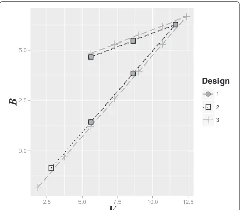
We considered three potential designs for the example in ‘Motivating example’. In Design 1, two interim analy-ses are planned, with the first occurring after a fixed 30 observations. Design 2 is similar, except that an additional earlier interim analysis is planned after 15 responses, with no early stopping for efficacy (u1 = ∞). In Design 3, six interim analyses are planned, where the first three are fixed at 10, 20 and 30 observations, with the first two analyses not allowing early stopping for efficacy (u1 =

u2= ∞).

We produced a graph of the boundaries for plotting the efficient score (Bi) versus Fisher’s information (Vi), and

for each design, investigated the operating characteris-tics by simulating 10,000 experiments under both the null and alternative hypotheses. Specifically, the Type I error, power and expected sample size were calculated.

Estimation of the probability of cure after extended follow-up

Consider estimating the probability of cure after extended follow-up (day 210) in the motivating example. For treat-mentj=1, 2, 3, the MLE is

ˆ

p210,j=S210,j/n210,j,

where S210,j denotes the number of successes (patients

cured) at day 210. If we focus on the treatmentj∗providing the apparent largest effect size, i.e.,

j∗=arg max

j=1,2,3pˆ210,j,

thenpˆ210,j∗is a biased estimate ofp210,j∗for two reasons.

Firstly, due to the potential early stopping of the trial based on the day 28 endpoint. Note that

ˆ

p210,j= ˆpjqˆj+(1− ˆpj)ˆsj (7)

wherepˆjdenotes the day 28 success proportion,qˆjdenotes

the proportion of patients who remain cured at day 210 (out of those already cured at day 28) andsˆjdenotes the

proportion of patients who switch from not cured at day 28 to cured by day 210 (out of those not cured at day 28, i.e., slow responders). It is well known that pˆj tends

to overestimatepj when a trial is stopped early for

effi-cacy (and underestimatepjwhen a trial is stopped early

for futility) [6], and this bias will be inherited bypˆ210,j. The

second source of bias is due to the multiple treatments being evaluated. Assuming that the success probabilities of the three treatments are reasonably similar, it is intu-itively clear that if we focus our attention on the largest success proportion, then this proportion will tend to be an overestimate.

We now investigate two methods that aim to improve estimation compared to the MLE. The first is a probabil-ity tree estimator (PTE), which attempts to address the

early stopping bias by replacingpˆj in (7) with a median

unbiased estimate. The second is a shrinkage estima-tor (SHE), which should help counteract both sources of bias by shrinking the three maximum likelihood estimates towards each other [12].

Probability tree estimator

In this PTE section, we omit the jsubscript to simplify the notation. Estimation of the success probability in the initial period, p, is subject to sequential stopping, while the subsequent follow-up is not. Hence, Omollo et al. proposed estimating the proportion with definitive cure— denoted by p210—using a probability tree argument to separate the two periods [7]. More specifically,p210is the sum of the probabilities of two events: (1) initial cure fol-lowed by cure at extended follow-up and (2) initial failure followed by cure during the extended follow-up. These probabilities are denotedpqand(1−p)s, respectively [pr

and(1−p)sin the notation of Omollo et al.], i.e.,qdenotes the conditional probability of cure at day 210 given cure at day 28, andsdenotes the conditional probability of cure at day 210 given no cure at day 28. Omollo et al. [7] proposed the following estimate forp210:

˜

p210= ˜pqˆ+(1− ˜p)ˆs,

where p˜ is the median unbiased estimate of p [6], with ˆ

q and ˆs being estimated by maximum likelihood from the 2 × 2 table of cure status at the two time points. The first term,p˜qˆ, takes into account those patients who relapse—important in VL trials. Here,qˆis the proportion of patients cured after treatment (at day 28 in Omollo et al.’s trial) who do not relapse. The second term,(1− ˜p)ˆs, accounts for slow responders—those who are not cured initially (at day 28) but become so by follow-up (day 210). Here,ˆsis the proportion of slow responders out of those patients who are not cured by day 28.

The sampling variance of this estimator was not derived by Omollo et al., so we do so here. We have

Var[p˜210]=Var[p˜qˆ]+Var[(1−˜p)ˆs]+2 Cov[p˜qˆ,(1−˜p)ˆs] .

The first two terms in the above expression can be ana-lyzed into variances of single parameters by using the standard formula for the variance of a product. We assume ˜

p,qˆandˆsare mutually independent. Denoting Var[p˜] by

σ2_{, and with an obvious notation for the variances ofqˆand} ˆ

sthen, for example, the first term becomes

For the third term, some expectation parameters can be taken into brackets:

2 Cov[p˜qˆ,(1− ˜p)ˆs]=2 E[p˜qˆ(1− ˜p)ˆs]−2 E[p˜qˆ] E[(1− ˜p)sˆ] =2 E[qˆ] E[ˆs]{E[p˜(1− ˜p)]

−E[p˜] E[(1− ˜p)]}

= −2 E[qˆ] E[ˆs]{E[p˜2]−(E[p˜])2} = −2 E[qˆ] E[ˆs]σ2.

Bringing the terms together, replacing the expectation by the observed values ofp˜,qˆ andsˆ, and gathering byσ_q2 andσ_s2yields:

Var[p˜210]=σq2

˜

p2+σ2+σ_s21− ˜p2+σ2+σ2(qˆ−ˆs)2. A 95 % confidence interval (CI) can then be calculated using

˜

p210±z1−α/2

Var p˜210

where z1−α/2 = 1.96 is the 1 − α/2 percentile of the standard normal distribution.

Shrinkage estimator

Shrinkage methods have a long and rich history in statis-tics, going back to the famous James–Stein estimator [13]. Their usefulness in the context of a clinical trial with mul-tiple treatment arms and interim analyses has been shown by Carreras and Brannath [12]. See also [14].

In very general terms, the idea is that the estimate of treatment effect in one particular group borrows infor-mation about the treatment effect in all other groups [15]. More specifically in our context, consider a probit transformation of the (day 210) success probabilities,

θj=−1_(p

210,j)forj=1, 2, 3,

wheredenotes the standard normal distribution func-tion. We now make the assumption that the success prob-abilities are similar to each other, in the sense that they have a common prior distribution that is Gaussian with meanμand varianceτ2_:

θj|μ,τ2∼N(μ,τ2), j=1, 2, 3.

This produces the effect that, compared to the maxi-mum likelihood estimateθjˆ = −1(pˆ210,j), the posterior mean ofθjis shrunk towardsμ—where the smallerτ2is, the greater the amount of shrinkage. In reality, we treat

μandτ2as unknowns and give them prior distributions. This produces the effect that the posterior means are shrunk towards each other, where the degree of shrink-age depends on how spread out the maximum likelihood estimates are. Our full model is

P(Yi,j=1)=p210,j, i=1,. . .,nj;j=1, 2, 3, (8)

p210,j=(θj), j=1, 2, 3, θj|μ,τ2∼N(μ,τ2), j=1, 2, 3,

μ∝1,

τ2_{∼IG(α,β),} α=2,

β=0.3,

where Yi,j is the day 210 response of theith patient on

treatment j, is the cumulative distribution function of the standard normal distribution andIG denotes the inverse-gamma distribution.

Our prior distribution forμis non-informative. How-ever, we do not choose a non-informative prior forτ, as this leads to problematic inferences when the number of groups is small [16]. Instead, we use an inverse-gamma distribution forτ2. The model (8) can then be fitted using a relatively simple Markov chain Monte Carlo (MCMC) algorithm [17], and we provide R code in the supplemen-tary material (see Additional file 1). The parameters of the inverse-gamma distribution are chosen based on our prior knowledge that a range of treatment effect sizes (θj’s) of−1_(0.9)−−1_{(0.75) ≈ 0.6 was very plausible, but a} range of effect sizes twice this large was fairly unlikely. For a normal distribution with variance 0.3, 42 % of the prob-ability density lies within 0.3 of the mean, and 73 % of the density lies within 0.6 of the mean. It, therefore, seemed a reasonable and pragmatic choice to giveτ2a prior mean of 0.3. This implies thatβ=0.3(α−1). Ifαis chosen too large, the degree of shrinkage or borrowing is effectively fixed in advance, i.e., it does not depend on how spread out the treatment effect estimates are. On the other hand, if α is too small, the MCMC will run into convergence issues. We, therefore, foundα=2 via a process of trial and error, such that the model gave acceptable performance in a range of simulated scenarios (see below).

The output of the MCMC algorithm is a sequence of draws θ_j(1),. . .,θ_j(N) from the posterior distribution of θj for j = 1, 2, 3. To produce a point estimate for p210,j, we take the mean of the back-transformed

draws

θ(1) j

,. . .,

θ(N) j

. A 95 % credible interval is found via the sample 2.5 % and 97.5 % quantiles of

θ(1) j

,. . .,θ_j(N).

Maximum likelihood estimator

As described previously, the MLE for the probability of cure after extended follow-up (day 210) in the motivating example is given by

ˆ

p210,j=S210,j/n210,j, j=1, 2, 3,

cured) andn210,j denotes the number of patients at day

210. A 95 % CI is then given by

ˆ

p210,j±z1−α/2

ˆ

p210,j(1− ˆp210,j)

n210,j

, j=1, 2, 3,

where z1−α/2 = 1.96 is the 1 − α/2 percentile of the standard normal distribution.

Bias and efficiency of the estimation methods

To compare the performance of the SHE, PTE and MLE, a simulation was performed to calculate bias, root mean square error (RMSE), length of 95 % CIs and coverage probabilities. We considered four different scenarios for the true proportion of successes at the end of treatment:

• Scenario 1: all treatments unpromising

p1=p2=p3=0.75

• Scenario 2: all treatments promising

p1=p2=p3=0.9

• Scenario 3: one treatment promising

p1=p2=0.75,p3=0.9

• Scenario 4: linear relationship between efficacy and treatment

p1=0.75,p2=0.825,p3=0.9

and four different cases for the change in patient status between the end of treatment and follow-up:

• Case 1: no relapses, no slow responders

q=1,s=0

• Case 2: no relapses, 33 % slow responders

q=1,s=0.33

• Case 3: 25 % relapses, no slow responders

q=0.75,s=0

• Case 4: 25 % relapses, 33 % slow responders

q=0.75,s=0.33

whereqandswere defined as for the PTE. For each com-bination of the above, 10,000 simulations of Design 2 were performed.

We calculated the bias and RMSE of the three estima-tors after selecting the best performing treatment of each simulation. The best performing treatment refers to the treatment with the largest estimated success probability at follow-up. The bias and RMSE from selecting the best treatment were calculated using the following formulas:

bias=bp(QS)=Ep(QS−pS)

and

RMSEp(QS)=

MSEp(QS)=

Ep (QS-p’S)2

=Varp(Qp)+b2_p(QS),

whereS ∈ (1, 2, 3)is the index of the selected treatment,

QS is the estimator used and p is the true value of the

efficacy at follow-up.

The length of the 95 % CIs is given as the upper confi-dence limit minus the lower conficonfi-dence limit. The cover-age probability of a CI gives the proportion of times the true value of the parameter (p) lies within the interval. For a 95 % CI, we would, therefore, expect the coverage probability to be approximately 0.95.

Trial registration and ethical approval

Ethical approval for the LEAP 0208 trial was obtained from the following committees: in Sudan, of the Insti-tute of Endemic Diseases, University of Khartoum (refer-ence IEND:UKIENDERC 2/11), and the Health Research Council, National Research Ethics Review Committee (reference 113-11-09), Ministry of Health of Sudan; in Kenya, of the Kenya Medical Research Institute (KEMRI EC, protocol 1720); and in the United Kingdom, of the London School of Hygiene and Tropical Medicine (refer-ence 5543). The trial is registered with ClinicalTrials.gov, number NCT01067443.

Results

Fixing an interim analysis after a pre-specified number of responses

Figure 3 shows the three potential designs for the moti-vating example. One can see that the boundaries become wider and the maximum sample size becomes larger as the number of interim analyses is increased. The results of the simulation exercise are summarized in Table 1. The

Table 1Parameter estimates for the three potential designs for the motivating example. A simulation was performed to calculate expected sample size, Type I error and power

Estimate Design 1 Design 2 Design 3

(3 analyses) (4 analyses) (7 analyses)

Maximum sample size 62 62 66

Expected sample size underH0 36 31 30

Expected sample size underH1 40 40 39

Type I error 0.0479 0.0482 0.0484

Power 0.893 0.889 0.894

expected sample size decreases as the number of interim analyses increases. Although all three designs satisfied the Type I error of 5 %, a power of 95 % was not achieved, with the average being approximately 90 %. This reduc-tion is due to the use of the normal approximareduc-tion, which has limited accuracy when used with a single stream of binary data and when used with success probabilities close to 1 (see p. 235 [10]). A simple correction is to increase the sample size until the simulated power exceeds 95 % (see Table 2). More accurate approaches are available that take explicit account of the binomial distribution of the data [18, 19].

Estimation of the probability of cure after extended follow-up

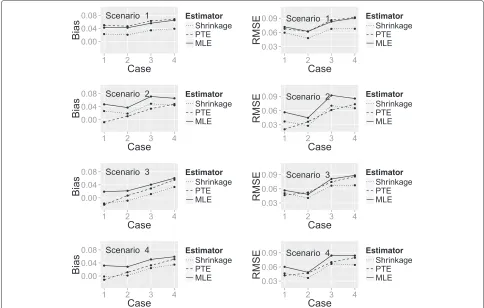
Figure 4 shows a plot of the bias and RMSE of the three estimators (SHE, PTE and MLE) calculated under each combination of the true success probability scenarios and change in patient status cases, with the latter represented on thex-axis. One can see that for all of the estimators, the bias and RMSE are higher for some scenarios than others. To some extent, this is explained by the closeness of the true probability to 1, which places an upper limit on the degree of the bias.

When all treatments are unpromising (Scenario 1), the SHE has the smallest bias and RMSE regardless of the change in patient status. In Scenario 2 (all treatments

Table 2Parameter estimates for the three potential designs for the motivating example under the maximum sample size required to satisfy power. A simulation was performed to calculate expected sample size, Type I error and power

Estimate Design 1 Design 2 Design 3

(3 analyses) (4 analyses) (7 analyses)

Maximum sample size 86 86 102

Expected sample size underH0 46 44 43

Expected sample size underH1 49 49 48

Type I error 0.0471 0.0453 0.044

Power 0.962 0.964 0.976

promising), the PTE has the smallest bias in all change of patient status cases. However, the performance of the estimators for RMSE differs dependent on the change in patient status. When there are no slow responders (patients not cured at end of treatment who become cured at extended follow-up), the PTE has the smallest RMSE; when there are slow responders, the SHE has the smallest RMSE.

When only one treatment is promising (Scenario 3) or when there is a linear relationship between efficacy and treatment (Scenario 4), the SHE has the smallest bias and RMSE in the majority of change in patient status cases. The PTE marginally outperforms the SHE when there is no change in patient status between the two time points.

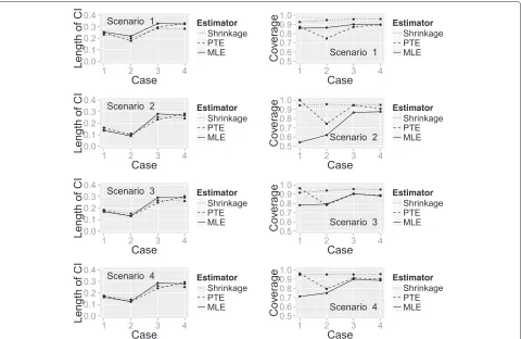
Figure 5 shows the length of 95 % CIs and the cover-age probability for the three estimators calculated under each combination of the true success probability scenar-ios and change in patient status cases, with the latter again represented on thex-axis. The length of the CIs is similar for all estimators whilst the coverage probability differs considerably between them. When all treatments are unpromising (Scenario 1), the SHE has much better coverage probability regardless of the change in patient status. In all other success probability scenarios, the SHE has the largest coverage probability in most cases, the exception being when there is no change in patient sta-tus between time points (Case 1) when the PTE performs better.

Discussion

Fixing an interim analysis after a pre-specified number of responses

The triangular test is a popular choice of sequential test due to its low expected sample size across a wide range of potential treatment effect sizes, and also for historical rea-sons, as very good approximations could be used to gen-erate stopping boundaries without a computer. We have shown how one can modify the triangular test to fix an interim analysis after a pre-specified number of patients. This enables a trial designer to guarantee the minimum number of patients necessary to obtain sufficient PK data unless a treatment is unpromising.

Just as for the standard triangular test, it remains true that the effect of increasing the number of interim analy-ses is to reduce the expected sample size, but at the price of increasing the maximum total sample size (see Table 1). A greater number of interim analyses provides more oppor-tunities to stop a trial early; however, it could make the trial less efficient to perform and increases the possibil-ity of overrunning—data accumulated after the formal stopping criterion has been reached (see Section 5.5 [6]).

Fig. 4Plot showing the bias and RMSE of the three estimators. A plot of bias and RMSE for the SHE, PTE and MLE calculated under each true success probability and change in patient status combination

For many types of non-normal data [6], they are achieved approximately. The adequacy of this approximation can be assessed via simulation. In our setting, we found that a Type I error of 5 % was achieved; however, a power of 95 % used in the trial designs was not achieved and the aver-age expected power was approximately 90 % (see Table 1). This reduction in power is due to the normal approxima-tion performing poorly with success probabilities close to 1 (see p. 235 [10]).

In this phase II trial, the emphasis was on learning rather than confirming, and therefore no formal correction was made for the multiple hypotheses tested.

Estimation of the probability of cure after extended follow-up

The second aim of the paper was to derive methods for estimation of the outcome variable (e.g., cure) at a time point later than that used for the stopping rule. In a trial for a new treatment approach for Indian VL [20], the impact of the group-sequential design was not considered in the analysis at the extended follow-up. Instead the MLE was used, which we know to be a biased estimator.

Simulation suggests that a SHE based on a Bayesian pro-bit model is the preferred choice of estimator (out of the SHE, PTE and MLE) for estimation of the probability of cure after extended follow-up. The simulation was per-formed under a range of true success probability scenarios and change in patient status cases (it is possible for there to be slow responders to treatment or relapses). The SHE performed best in most situations in terms of reducing both bias and RMSE and providing coverage probabilities close to 0.95. The PTE performed well in instances where there was no change in patient status between end of treat-ment and follow-up. The MLE was poor in all instances. It is well known that for binary data, the MLE CI based on the normal approximation only performs well for large

n. Agresti states that “the actual coverage probability usu-ally falls below the nominal confidence coefficient, much below whenπis near to 0 or 1”, whereπ is the true suc-cess proportion [21]. We would not recommend using the MLE for estimation of efficacy at follow-up based on these findings in any of the scenarios considered.

Fig. 5Plot showing the length of 95 % CIs and coverage probability of the three estimators. A plot of the length of 95 % CIs and coverage probability for the SHE, PTE and MLE calculated under each true success probability and change in patient status combination

effects is a subtle task. The SHE would also be unsuitable for use in trials of a single treatment arm and so the PTE may provide a suitable alternative.

Conclusions

Generalization of the triangular design is simple to imple-ment and allows the minimum number of patients neces-sary for PK analysis to be obtained. For the estimation of efficacy at follow-up following a sequential design trial, a SHE is preferable. The PTE would provide an alternative for use in one-arm trials or when the SHE is not possible due to its computational complexity.

Additional file

Additional file 1: Supplementary R functions.Zip file containing all R code necessary to reproduce our results, together with description files that explain how to use the functions. Installation instructions can be found at: http://cran.r-project.org/doc/manuals/r-release/R-admin.html# Installing-packages. (PDF 463 kb)

Abbreviations

CI: confidence interval; MCMC: Markov chain Monte Carlo; MLE: maximum likelihood estimator; PK: pharmacokinetic; PTE: probability tree estimator; RMSE: root mean square error; SHE: shrinkage estimator; VL: visceral leishmaniasis.

Competing interests

The authors declare that they have no competing interests.

Authors’ contributions

AA derived the symmetric and asymmetric modified boundaries. NA derived the estimator for the sampling variance of the probability tree approach, and expressed general forms for the modified boundaries. DM contributed code for evaluating the performance of the estimation procedures. AA wrote the first draft of the manuscript. AA, TE, RO, FA, DM and NA edited the manuscript. All authors read and approved the final manuscript.

Acknowledgments

TE receives salary support from the Drugs for Neglected Diseases Initiative (DNDi), the Medical Research Council and the Department for International Development (MR/K012126/1). NA receives salary support from the DNDi. Dominic Magirr was supported by the Austrian Science Fund, (FWF) Fonds zur Förderung der wissenschaftlichen Forschung (Project P23167).

Author details

1_{Lancaster University, LA1 4YW Lancaster, UK.}2_{The University of Sheffield,}

Western Bank, S10 2TN Sheffield, UK.3MRC Tropical Epidemiology Group, London School of Hygiene and Tropical Medicine, Keppel Street, WC1E 7HT London, UK.4Drugs for Neglected Diseases initiative (DNDi) Africa, Centre for Clinical Research, Kenya Medical Research Institute, Nairobi, Kenya.5_Maseno

University, Private Bag, Maseno, Kenya.6DNDi, Geneva, Switzerland.7Centre for Medical Statistics, Medical University of Vienna, Spitalgasse 23, 1090 Vienna, Austria.

References

1. Alvar J, Vélez I, Bern C, Herrero M, Desjeux P, Cano J, et al. Leishmaniasis worldwide and global estimates of its incidence. PloS One. 2012;7(5): 35671.

2. Musa A, Khalil E, Hailu A, Olobo J, Balasegaram M, Omollo R, et al. Sodium stibogluconate (SSG) & paromomycin combination compared to SSG for visceral leishmaniasis in East Africa: a randomised controlled trial. PLoS Negl Tropical Dis. 2012;6(6):1674.

3. van Griensven J, Balasegaram M, Meheus F, Alvar J, Lynen L, Boelaert M. Combination therapy for visceral leishmaniasis. Lancet Infect Dis. 2010;10(3):184–94.

4. Olliaro P, Vaillant MT, Sundar S, Balasegaram M. More efficient ways of assessing treatments for neglected tropical diseases are required: innovative study designs, new endpoints, and markers of effects. PLoS Negl Tropical Dis. 2012;6(5):1545.

5. Sébille V, Bellissant E. Sequential methods and group sequential designs for comparative clinical trials. Fundam Clin Pharmacol. 2003;17(5):505–16. 6. Whitehead J. The design and analysis of sequential clinical trials. In:

Statistics in practice. Chichester: John Wiley & Sons; 1997.

7. Omollo R, Alexander N, Edwards T, Khalil E, Younis BM, Abuzaid A, et al. Safety and efficacy of miltefosine alone and in combination with sodium stibogluconate and liposomal amphotericin B for the treatment of primary visceral leishmaniasis in East Africa: study protocol for a randomized controlled trial. Trials. 2011;12(1):166.

8. Ranque S, Badiaga S, Delmont J, Brouqui P. Triangular test applied to the clinical trial of azithromycin against relapses inPlasmodium vivax infections. Malar J. 2002;1:13.

9. Cox DR, Hinkley DV. Theoretical statistics. London: Chapman Hall; 1974. 10. Jennison C, Turnbull BW. Group sequential methods with applications to

clinical trials. Florida: CRC Press; 1999.

11. Whitehead J. Group sequential trials revisited: simple implementation using SAS. Stat Methods Med Res. 2011;20(6):635–56.

12. Carreras M, Brannath W. Shrinkage estimation in two-stage adaptive designs with midtrial treatment selection. Stat Med. 2013;32(10):1677–90. 13. James W, Stein C. Estimation with quadratic loss. In: Proceedings of the

4th Berkeley Symposium on Mathematical Statistics and Probability. Berkeley, California: University of California Press; 1961. p. 361–79. 14. Bowden J, Brannath W, Glimm E. Empirical bayes estimation of the

selected treatment mean for two-stage drop-the-loser trials: a meta-analytic approach. Stat Med. 2014;33(3):388–400. 15. Berry SM, Broglio KR, Groshen S, Berry DA. Bayesian hierarchical

modeling of patient subpopulations: efficient designs of phase II oncology clinical trials. Clin Trials. 2013;10(5):720–34.

16. Gelman A. Prior distributions for variance parameters in hierarchical models (comment on article by Browne and Draper). Bayesian Anal. 2006;1(3):515–34.

17. Albert JH, Chib S. Bayesian analysis of binary and polychotomous response data. J Am Stat Assoc. 1993;88(422):669–79.

18. Stallard N, Todd S. Exact sequential tests for single samples of discrete responses using spending functions. Stat Med. 2000;19(22):3051–64. 19. McWilliams TP. An algorithm for the design of group sequential triangular

tests for single-arm clinical trials with a binary endpoint. Stat Med. 2010;29(27):2794–801.

20. Sundar S, Rai M, Chakravarty J, Agarwal D, Agrawal N, Vaillant M, et al. New treatment approach in Indian visceral leishmaniasis: single-dose liposomal amphotericin B followed by short-course oral miltefosine. Clin Infect Dis. 2008;47(8):1000–6.

21. Agresti A, Vol. 359. Categorical data analysis. Hoboken: John Wiley & Sons; 2002.

Submit your next manuscript to BioMed Central and take full advantage of:

• Convenient online submission

• Thorough peer review

• No space constraints or color figure charges

• Immediate publication on acceptance

• Inclusion in PubMed, CAS, Scopus and Google Scholar

• Research which is freely available for redistribution