Towards A Promising Edge Classification Algorithm for the Graph Isomorphism Problem

(1)

G

Gd

Towards a Promising Edge Classification Algorithm for

the Graph Isomorphism Problem

Islam A.T.F.Taj-Eddin

Faculty of Informatics and Computer Science, The British

University in Egypt, Cairo, Egypt.

Samir Abou El-Seoud

Faculty of Informatics and Computer Science, The British

University in Egypt, Cairo, Egypt.

Jihad M. AL-Ja’am

College of Engineering, Dept. of Computer Science

and Engineering, Qatar University, Qatar.

ABSTRACT

For over three decades the Graph Isomorphism (GI) problem has been extensively studied by many researchers in algorithms and complexity theory. To date, there is no formal proof to classify this problem to be in the class P or the class NP. In this paper, evidence had been proposed of the existing of polynomial time algorithm based on edge classification which can be used to prove that GI is rather in the class P.

General Terms

Computational Mathematics, Theoretical Informatics, Theoretical Computer Science, Graph Algorithms, Algorithms.

Keywords

Edge Classification, Graph Isomorphism, Polynomial Algorithm, Graph Canonization.

Nomenclature

GI Graph isomorphism Gd Directed Graph

DG Directed unweighted graph with no self-loops and no multiple edges

SnD Square n-partite directed acyclic graph EBFS Edge Breadth First Search

1. INTRODUCTION

The Graph Isomorphism (GI) problem consists of deciding whether two given graphs are identical even if they look different in their graphical or adjacency matrices representation. Formally, two graphs G1 and G2 are called isomorphic if there is a bijection function b from the vertex-set V1 of G1 to the vertex-vertex-set V2 of G2 such that the edge (vi,vj) belongs to G1 if and only if the edge (b(vi),b(vj)) belongs to G2 and b is an isomorphism [10]. The problem has many applications in different fields, such as in cheminformatics [15], graphical data mining [9] and electronic design verification [5]. Even though, the GI problem has remarkable properties in terms of its complexity structure, it is still not known whether it is in the class P, or the class NP (assuming that P ≠ NP). However, there is some evidence to support that GI is not an NP-complete problem. In fact, if it is in NP then the polynomial hierarchy would collapse to the second level [17][6]. In addition, GI is also not known to be hard for P. In fact, the best known hardness results are still relatively weak [19][1][17].

More formally, two graphs G1 and G2 are isomorphic if they have the same number of vertices, the same number of edges, the same degree sequence for the vertices, and the same edges

could be tested in a polynomial time. Without any loss of generality, the graphs G1 and G2 have the same number of vertices, the same number of edges and the same degree sequences. The fourth condition is relatively hard to be tested. It could be shown that there exists two graphs that satisfy the first three conditions but do not have isomorphic set of consistently generated trees (i.e. they do not satisfy the fourth condition) [17]. It is sufficient and enough to generate all possible paths of length at most n, where n is the number of vertices in both graphs G1 and G2, to prove the isomorphism of G1 and G2 based on the isomorphism of all possible generated paths. This could be done in an exponential time at the worst case.

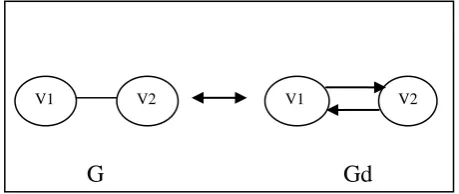
We assume that the graphs G1 and G2 are connected, unweighted, undirected and their vertices have no self-loops. In this paper, an undirected graph G will be represented by its corresponding Directed Graph (Gd), such that every undirected edge between the vertices v1 and v2 of G will be replaced by two directed edges in Gd. The first edge is from v1 to v2 while the second edge is from v2 to v1. Figure 1 shows an example.

[image:1.595.315.545.543.640.2]

Note that the adjacency matrices of G and Gd are clearly identical. Then the undirected graphs G1 and G2 will be replaced by their corresponding directed graphs Gd1 and Gd2. The isomorphism problem between G1 and G2 will be transformed to the problem of finding the isomorphism between Gd1 and Gd2.

Fig. 1: The undirected graph G is represented by its corresponding directed graph Gd.

2. PREVIOUS WORKS

Unlike general graphs, it has been shown that there exists an efficient solution for the GI problem for special graphs with specific constraints on the number of vertices and edges (i.e. trees, planar graphs, permutation graphs, graphs of bounded degree) [16][14][8][20][13].

The graph canonization is the essence of many graph

(2)

is some canonizing function for graphs that can be computed in polynomial time, and if the two problems are polynomial-time equivalent [3][4][1][17][18][12].

Many attempts, of different nature, have been made to establish the GI complexity status. According to the current knowledge, there is no formal proof to solve the GI problem in a polynomial time. An attempt of using the edge classification algorithm to classify the GI problem was introduced in the late sixties [22][21]. Even though, it didn’t provide a general formal proof, it succeeded however to classify GI for several types of graphs [2]. Note that, it has been proved in [7] that edge classification and n-tuples classification algorithms were unable to distinguish among all pairs of non isomorphic graphs. In [7], they considered graphs of O(n) distinct vertices, with color class size of 4, and assumed a linear time canonical labeling algorithm. The resulted canonical form of the graph is isomorphic to its corresponding graph.

In [11], it has been mentioned that:

"….if f is an isomorphism between H and G itself, then any change in G must be reflected by a corresponding change in H, or else f will no longer be an isomorphism. In other words, proofs of NP-completeness seem to require a certain amount of redundancy in the target problem, a redundancy that GRAPH ISOMORPHISM lacks. Unfortunately, this lack of redundancy does not seem to be much of a help in designing a polynomial time algorithm for GRAPH ISOMORPHISM either, so perhaps it belongs to NPI…"

In this work, an edge classification algorithm that can be used to classify GI problem to be rather in the class P has been presented. The paper edge classification algorithm doesn’t run against the proof given in [7]. In fact, the resulted canonical labeling graph, presented in this paper, contains redundant (not distinct) vertices. The element of redundancy will be used later, as a constraint, in the isomorphism testing without contradicting [7] (see figure 3 and theorem 2). The resulted canonical labeling graph is not isomorphic to its corresponding graph, yet it is a one-to-one and onto transformation.

3. GRAPH CANONIZATION

In this section, a vertex v of one graph will be chosen. The edges will be classified according to their distance from v. The classification procedure is presented as a (one-to-one and onto) transformation from the input graph (Gd) to an output graph denoted by SnD (the square n-partite directed acyclic graph) allowing the representation of paths of minimal length between the initial vertex v and all other vertices. The resulted graph (SnD) is not isomorphic to the original graph (Gd). Theorem 1 and its proof summarize the idea.

We assume that there exists a given starting vertex for any given graph Gd and for any directed unweighted graph with no self-loops and no multiple-edges (DG). Any criteria could be used to choose the starting vertex. Since Gd DG, then the work will be done first with DG and later with Gd.

A square n-partite directed acyclic graph of n n vertices (SnD), is an ordered finite set S of tuples Sj, where S = {Sj | 1 ≤ j ≤ n} and n is the number of vertices in DG, such that the following four rules must be satisfied:

1. The tuple Sj, 1 ≤ j ≤ n, is a finite collection of distinct n vertices, Sj=(vi | 1 ≤ i ≤ n).

2. Tuples Sj, 1 ≤ j ≤ n, are equal (i.e. S1=S2=S3=…..=Sn).

3. Vertices of Sj, has a direct relation only with vertices of Sj+1, 1 ≤ j ≤ n-1.

This direct relation is written as an ordered pair (vxj,vy(j+1)), with 1≤x,y≤n, x y, (i.e. vxj is vertex vx that is a member of Sj and has a direct relation with vy(j+1) which is vertex vy that is a member of Sj+1).

4. For any x and y, 1≤x,y≤n, if there exists a direct relation between vx and vy then there exists one and only one tuple (vxi,vy(i+1)), 1 ≤ i ≤ n-1. This means that if there exists (vx3,vy4) then it is prohibited to have (vxi,vy(i+1)), such that (1 ≤ i ≤ n-1and i 3). (i.e, if (vx3,vy4) is true, then it is prohibited to have (vx1,vy2),(vx2,vy3), (vx4,vy5),…..,(vx(n-1),vyn)).

3.1 Example 1

Assuming a square 3-partite SnD with a certain order as S={S1=(v1,v3,v2),S2=(v1,v3,v2),S3=(v1,v3,v2)}.

By rule 1 and 2, it could be written as S={(v11,v31,v21), (v12,v32,v22), (v13,v33,v23)}, see figure 2. By rule 3, (v11,v22), (v11,v32) are allowed while (v11,v12), (v11,v23) are prohibited. By rule 4, if (v11,v32) does exist then (v12, v33) is prohibited.

Fig. 2: The graph representation of S={(v11,v31,v21),(v12,v32,v22),(v13,v33,v23)}.

3.2 Definition 1

Definition 1: Let Gs denotes the set of (vx,DG), vx is the starting vertex of DG, 1≤x≤n, n is the number of vertices in DG. Let Gt denotes the set of (vx1,SnD), vx1, which is the vertex vx that is a member of S1 of SnD, is the starting vertex of SnD.A canonical function for Gs is a one-to-one and onto function f (f: Gs Gt) from Gs to Gt, f(vx,DG) = (vx1,SnD) and f-1(vx1,SnD)= (vx,DG), such that the (vx1,SnDi) is isomorphic to (vy1,SnDj) if and only if (vx,DGi) is isomorphic to (vy,DGj).

Next, a one-to-one (f) and onto (f)-1 canonical functions that respect definition 1 will be proposed.

V11 V31 V21

V12 V32 V22

(3)

We define the function (f) as follows:

1. The input is a directed graph DG with a starting vertex vx.

2. We have f(vx,DG) =(vx1,SnD).

3. The output is SnD with a starting vertex vx at tuple S1 (i.e. vx1).

We apply (f) as follows:

1. The input is (vx,DG)

2. Apply (EBFS(vx,DG))

Edge-Breadth-First-Search (EBFS), is similar in execution mechanism, correctness and time complexity to Breadth-First-Search (BFS) [10], but differs in the following:-

EBFS(vx,DG)

1. The input is a directed graph DG with a starting vertex vx.

2. The distance value (d) will be assigned to each edge rather than to each vertex. The distance value of the edge indicates how far is the edge on a path taken starting from the vertex vx. Each edge traversed exactly once, and a distance value (d) is assigned to it.

3. The output is a directed graph DG with a starting vertex vx and a distance value (d) for each edge, 1≤d≤n.

3. Create an Empty SnD, as stated at the definition of SnD n is the number of vertices in DG used in the previous steps. For each directed edge e=(vy,vz) with distance (d) in DG, set a direct edge from vy that belongs to set S(d) to vz that belongs to set S(d+1) (i.e. (vy(d),vz(d+1))).

4. Output SnD with starting vertex vx at tuple S1 (i.e. vx1).

We conclude that f(vx,DG) =f(EBFS(vx,DG))= (vx1,SnD).

We define (f) -1 as follows:

1. The Input is SnD with a starting vertex vx at tuple S1 (i.e. vx1).

2. f-1 (vx1,SnD)=(vx,DG).

3. The output is a directed graph DG with starting vertex vx.

Apply (f) -1 as follows:

1. The input is SnD with starting vertex vx at tuple S1 (i.e. vx1).

2. Create an empty DG with n vertices. For each directed edge e=(vy(d),vz(d+1)), set a direct edge from vy to vz with one distance (d) for the edge in DG. Delete the value of (d) from each edge.

3. The output is a directed graph DG with a starting vertex vx.

We conclude that f-1 (vx1,SnD)= f -1

(EBFS(vx,DG))= f -1

(vx,DG)= (vx,DG).

3.3 Theorem 1

Theorem 1: The function (f) is a one-to-one and onto function, such that:

1. f(vx,DG)=(vx1,SnD). 2. f-1_(v

x1,SnD)= (vx,DG).

Proof:

1. In order for (f) not to be one-to-one, the following equations must be true:-

f(vx,DG)=f(EBFS(vx,DG))=(vx1,SnD1) and f(vx,DG)=f(EBFS(vx,DG))=(vx1,SnD2),

Assume that SnD1 SnD2, there must exist a directed edge e=(vy,vz) with distance (d) in DG, such that there exists a direct edge from vy at set S(d) to vz at set S(d+1) (i.e. (vy(d),vz(d+1))) at SnD1 and a different direct edge from vy at set S(d) to vz at set S(d+1) (i.e. (vy(d),vz(d+1))) at SnD2.

Since the edge e=(vy,vz) has one and only one value for (d), the edge e=(vy,vz) with distance (d) at SnD1 and e=(vy,vz) with distance (d) at SnD2 will be equal in distance (d) and position. The same could be said about all other edges, which means SnD1= SnD2 (contradiction).

2. In order for f-1 not to be onto, the following equations must be true:- f-1 (vx1,SnD)= f-1 (EBFS(vx,DG1)) = (vx,DG1) and f

-1

(vx1,SnD)= f -1

(EBFS(vx,DG2)) = (vx,DG2)

Assume that DG1 DG2, there must exist a directed edge e=(vy(d),vz(d+1)), such that there exists a direct edge from vy to vz with distance (d) at DG1 and a different direct edge from vy to vz with distance (d) at DG2. Since the edge e=(vy(d),vz(d+1)) is corresponding to one and only one edge e=(vy,vz) with distance (d), the edge e=(vy,vz) with distance (d) at DG1 will be equal with the edge e=(vy,vz) with distance (d) at DG2. The same could be said about all other edges, which means DG1= DG2 (contradiction).

4. THE RELATIONSHIP BETWEEN

Gd1, Gd2 AND SnD1, SnD2

From now on and without any loss of generality, the paper will only deal with the Gd that represents a connected unweighted and undirected graph G.

As stated earlier, if and only if there is an algorithm to discover the isomorphism between SnD1 and SnD2 that will enforce that Gd1 is isomorphic to Gd2 and vise versa. (i.e. G1 Gd1 SnD1, and G2 Gd2 SnD2).

(4)

between SnD1 and SnD2 lies in the fact that SnD graph is sharing some common characteristics with planar graphs. An efficient polynomial time algorithm that can discover isomorphism between planar graphs was given in [16][14][8][20][13]. By definition, SnD1 does not have K5. By definition, SnD1 has V=n2 vertices and maximum of E=n2 -n edges. E = -n2_-n _3V2 _{– 6), for n}2 _{3, and E = n}2_-n

(2V2- 4), for n2 3 [16][14][8][20][13]. In spite of these common characteristics with planar graphs, the graph SnD considered here is not a planar graph.

Before trying to discover a polynomial time algorithm for isomorphism between SnD1 and SnD2, a proof should be given for the case of any two distinct graphs Gd1 and Gd2 it holds that SnD1 and SnD2 differ at least in one characteristic of one metric. A definition of SnD metric will be given followed by a theorem and its proof.

4.1 Definition 2

Definition 2: define the metric sg(vi,ki) as the ordered finite tuple (vi1,vi2,vi3,…..,vin), for 1 i n that belongs to SnD, ki, 1 ki n, is the location of vi within all tuples S. It is allowed for a whole metric to swap with another whole metric only.

There exist some characteristics on metrics sg(vi,ki), for 1 i n. These characteristics are:

in-degree(viy) is the number of edges coming from any other vertex to vertex viy,

out-degree(viy) is the number of edges coming into any other vertex from vertex viy,

from-to(viy) is the ordered tuple of location(s) kj, such that an edge is coming from vertex (viy), which belongs to the metric sg(vi,ki), going to vertex (vjx) which belongs to the metric sg(vj,ki) (i.e. (viy)(vjx)).

4.2 Example 2

Assuming a square 3-partite SnD is:

S={S1=(v1,v3,v2), S2=(v1,v3,v2), S3=(v1,v3,v2)}, that could be written as S={(v11,v31,v21), (v12,v32,v22), (v13,v33,v23)}.

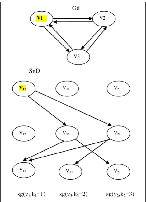
Assuming the starting vertex is v11, see figure 3. The characteristics on metric sg(vi,ki) of figure 3 are as follows:

metric sg(v1,k1=1)=(v11,v12,v13):

in-degree(v11)=0 ,

out-degree(v11)=2,

from-to(v11)=(k3=2,k2=3),

from-to(v12)= Ø,

from-to(v13)= Ø.

metric sg(v2,k2=3)=(v21,v22,v23):

from-to(v22)=(k1=1,k3=2),

metric sg(v3,k3=2)=(v31,v32,v33):

in-degree(v31)=0,

from-to(v32)=(k1=1,k2=3),

4.3 Theorem 2

Theorem 2: Given the set of all metrics computed for SnD1 of Gd1 and SnD2 of Gd2, it holds that if and only if Gd1 and Gd2 are distinct then SnD1 and SnD2 will differ at least in one characteristic of one metric.

Proof:

1. (If) Gd1 and Gd2 are distinct then SnD1 and SnD2 will differ at least in one characteristic of one metric.

1.1. It is sufficient and enough to generate all possible paths of length at most n, beginning from a certain vertex vx, where n is the number of vertices in both graphs Gd1 and Gd2, to prove the isomorphism of Gd1 and Gd2 based on the isomorphism of all possible generated paths. That could be done in exponential time at worst case analysis.

(5)

Gd

SnD

sg(v1,k1=1) sg(v3,k3=2) sg(v2,k2=3)

[image:5.595.52.287.76.401.2]

Fig. 3: This is the resulted SnD, with the starting vertex v11, from the corresponding directed graph Gd, with the

starting vertex v1, such that

Gd={(v1,v2),(v2,v1),(v1,v3),(v3,v1),(v2,v3),(v3,v2)}, ki is the

location of the metric sg(vi,ki)=(vi1,vi2,vi3), 1≤ki≤3.

1.3. If Gd1 and Gd2 are distinct then:

1.3.1. Either at least one path, of the subset of the generated all possible paths, has different length at Gd1 than Gd2. For that case, it could be shown that at least one metric at SnD1 has different characteristic ( in-degree(viy),out-degree(viy),

from-to(viy)) than SnD2;

1.3.2. Or all paths have the same length, but at least one path, of that subset of the generated all possible paths at Gd1, has different relations (i.e. no bijection) than any paths at Gd2.

For that case, metrics at SnD1 and SnD2 will have the same ( in-degree(viy),out-degree(viy)) characteristics, but at least one metric at SnD1 will be different in its (from-to(viy)) characteristic than any metric at SnD2.

Because since the paths length are equal in both Gd1 and Gd2, then (in-degree(v ),out-degree(v ))

characteristics in SnD1 and SnD2 will not be enough to distinguish between them, but from the definition of isomorphism no bijection means there exist at least one edge between two vertices in Gd1 that has no match in Gd2, that case will manifest itself at the ( from-to(viy)) characteristic which catch that relation between vertices of metrics in SnD1.

From the definition of isomorphism, the (from-to(viy)) characteristic of one metric in SnD1 will be different than any (from-to(viy)) characteristic of any metric in SnD2.

2. (Only if) SnD1 and SnD2 differ at least in one characteristic of one metric then Gd1 and Gd2 are distinct. That could be deduced directly from f-1 of Theorem 1.

5. CONCLUSION AND FURTHER

WORK

The GI problem is extremely relevant in theoretical computer science. Many attempts, of different nature, have been made to establish its complexity status. Among these attempts, the classification of tuples of vertices is an important one. An edge classification algorithm that can be used to prove that GI problem is rather in the class P will be presented. The proposed algorithm chooses a vertex v of one graph and classifies the edges according to their distance from that vertex v. The classification procedure is presented as a transformation from the input graph Gd to a directed graph SnD allowing the representation of paths of minimal length between the initial vertex and all other vertices. The transformed graph SnD is not isomorphic to the original graph Gd. The proposed approach introduces the element of redundancy that does not contradict with the work given in [7].

As further work, a polynomial time algorithm that shows SnD1 is isomorphic to SnD2 is worth the trial to be found. Based on Theorem 2, if and only if Gd1 and Gd2 are distinct then SnD1 and SnD2 will differ at least in one characteristic of one metric. One reason behind the believe of the existence of a polynomial time algorithm that can discover isomorphism between SnD1 and SnD2 lies in the fact that SnD graph sharing some common characteristics with planar graphs. In spite of these characteristics, SnD is not a planar graph.

6. ACKNOWLEDGMENTS

The authors would like to thank Dr. Khaled Nagati, and all of the academic staff of the Faculty of Informatics and Computer Science at the BUE for their valuable remarks and suggestions.

7. REFERENCES

[1] Arvind V., and Toran J. 2005. Isomorphism Testing: Perspective and Open Problems, Bulletin of the European Association for Theoretical Computer Science, Computational Complexity Column, (June, 2005), Number 86.

V11 V31 V21

V12 V32 V22

V13 _V₃₃ _V₂₃

V1 V2

(6)

[2] Babai L. 1996. Automorphism groups, isomorphism, reconstruction, Handbook of Combinatorics (eds. R. L. Graham, M. Grotschel and L. Lovasz), Chapter 27, North-Holland, Amsterdam, (1996), pages 1447-1540.

[3] Babai L. and Kucera L. 1979. Canonical labeling of graphs in average linear time. Proc. 20th Annual IEEE Symposium on Foundations of Computer Science, 1979, 39–46.

[4] Babai L. and Luks M. 1983. Canonical labeling of graphs. In proceedings of the fifteenth annual ACM symposium on theory of computing, 1983, page 171-183.

[5] Baird H.S., Cho Y.E. 1975. An artwork design verification system, Proceedings of the 12th Design Automation Conference. IEEE Press., (1975) , pp. 414-420.

[6] Boppana R., Hastad J. and Zachos S.1987.Does co-NP have short interactive proofs?, Information Processing Letters 25(2), (1987), pages 127-132.

[7] Cai J., Furer M., and Immerman N. 1992. An optimal lower bound on the number of variables for graph identification. Combinatorica, 12:389-410, (1992).

[8] Colbourn C.J. 1981. On testing isomorphism of permutation graphs, 1981, Networks 11: 13–21, doi:10.1002/net.3230110103.

[9] Cook D. J. and Holder L. B. 2007. Mining Graph Data, John Wiley & Sons, 2007.

[10]Cormen T. H., Leiserson C. E., Rivest R. L. and Stein C. 2009. Introduction to algorithms, 3rd edition, the MIT press, 2009.

[11]Gary M. R. and Johnson D. S. 2000. Computers and Intractability a Guide to the Theory of NP-Completeness, W.H. FREEMAN AND COMPANY, NY, 1979, pp. 155-156.

[12]Gurevich Y. 1997. From Invariants to Canonization, The Bulletin of European Association for Theory of Computer Science, 1997, Number 63.

[13]Hopcroft J. and Tarjan R. E. 1974. Efficient planarity testing. J. ACM, (1974), 21(4):549–568.

[14]Hopcroft J. and Wong J. 1974. Linear time algorithm for isomorphism of planar graphs, Proceedings of the Sixth Annual ACM Symposium on Theory of Computing, 1974, pp. 172–184, doi:10.1145/800119.803896.

[15]Irniger C-A M 2005. Graph Matching: Filtering Databases of Graphs Using Machine Learning, Aka, 2005.

[16]Kelly P.J. 1957. A congruence theorem for trees, Pacific J. Math., 7, 1957, pp. 961–968.

[17]kobler J., Schoning U., and Toran J. 1993. The graph isomorphism problem: Its structural complexity. Birkhauser, 1993.

[18]McKAY B. D. 1981. Practical Graph Isomorphism. Congr. Numerantium ,(1981), 30, 45-87. (Nauty User’s Guide, Version 2.2 (beta 6); (2003) (http://cs.anu.edu.au/people/bdm/nauty/)).

[19]Toran J. 2000. On the hardness of graph isomorphism. FOCS, 2000, 180–186.

[20]Toran J. and Wagner F. 2009. The complexity of planar graph isomorphism, Bulletin of the European Association for Theoretical Computer Science, Computational Complexity Column, (February 2009), Number 97.

[21]Weisfeiler Boris ed. 1976. On Construction and Identification of Graphs, Lecture Notes in Mathematics 558, Springer, (1976).