Fault Localization using Probabilistic Program Dependence Graph

Fault Localization using Probabilistic Program

Dependence Graph

N.Suguna

Computer Science and Engineering, Annamalai University,

Chidambaram, Tamilnadu, India.

R M. Chandrasekaran, PhD.

Annamalai University, Chidambaram, Tamilnadu, India

.

ABSTRACT

Fault localization is an expensive technique in software debugging. Program dependence graphs are used for testing, debugging and maintenance applications in software engineering. Program dependence graphs (PDG) are used to build a probabilistic graphical model of program behavior. In this paper we proposed a model based fault localization technique using probabilistic program dependence (PPDG).This work presents algorithm for constructing PPDGs and PPDGs based fault localization. Our experimental result shows that proposed PPDG based fault localization method performs better than existing testing based fault localization (TBFL) method for DotNet programs. Our results also indicate that the probabilistic approach is efficient for fault localization.

Keywords

Probabilistic Program Dependency Graph, Program Dependency Graph, Testing Based Fault Localization, Conditional Probabilistic Table.

1. INTRODUCTION

In debugging, the programmers have to remove the bug part of the program without introducing new bugs at the same time. However fault localization is difficult and time consuming process there are several testing tools available. In order to reduce the cost of debugging several automated testing tools based on techniques such as static, dynamic and execution slice based, spectrum based, statistics based, program state based, machine learning based, similarity based and model based technique are used [2, 6, 8,9,11,13,15].

Program dependence Graph is a combination of control flow graph and data flow graph. With the help of PDG, a PPDG is constructed. PPDG is a conditional statistical dependence model which depicts the independence relationships among program elements.

Our proposed work identifies the internal behavior for a set of test inputs. It uses the program dependency graph to estimate the statistical dependencies between node states for a set of test inputs for fault localization. We compare the TBFL [4] and PPDG technique. The result shows that PPDG is more effective than TBFL.

Section 2 describes the different existing fault localization techniques. Section 3 explains about fault localization using TBFL. Section 4 defines PPDG construction. Section 5 and 6 discuss about fault localization techniques used. Section 7 describes the performance comparison results between TBFL and PPDG and section 8 defines conclusion.

2. RELATED WORK

Fault Localization is a complex and time consuming process. There are several techniques for fault localization. The first technique was introduced by Mark Weiser named as slicing. A slice is an executable set of statements which preserves the original behavior of the program with respect to a subset of variables at a given program point [16]. In [4] the author proposed an efficient dynamic slicing algorithm for debugging, program integration software maintenance and reverse engineering [4].

Program spectrum based technique identifies the suspicious statement in a program responsible for failure. It records the execution information to find the success or failure of a statement [5]. The disadvantage of this method is does not differentiate the cause of a successful or failed testcase. Renieris & Reiss presents a spectrum based technique which contrasts the failed test case with successful test case [6].

Statistics based fault localization technique finds the fault in the program by contrasting the statistics of the evaluation results of individual predicates between failed runs and successful runs. It uses the short circuit evaluations to improve predicate based statistical fault localization techniques[7].

Liblit et al. proposed a statistical debugging algorithm to identify bugs in the programs with instrumented predicates at particular points [8]. Feedback reports are generated by these instrumented predicates. Predicates with a higher score should be examined first to find bugs. Once a bug is found and fixed, the feedback reports related to that particular bug are removed. This process is continued until other bugs and all the feedback reports are removed or all the predicates are examined.

W.Eric .Wong uses the neural network to locate the bugs effectively. It identifies the relationship between the statement coverage information of a test case. It uses this information for success or failure of a test case[9]. Wong et al. [10] also proposed a crosstab method to find the suspiciousness of each executable statement in terms of its likelihood of containing program bugs.

association rules and Formal concept Analysis to assist in fault localization

The main objective of our work is to develop a model based fault localization method. We generate the PPDG for Dotnet programs. Then the PPDG generated is used for localizing the faults in our input test cases. The results are compared with TBFL to show the effectiveness of PPDG based approach.

3. FAULT LOCALIZATION USING TBFL

In order to reduce the cost of debugging, fault localization techniques are automated. One such technique used in TBFL which is based on information gathered from testing. Given a program which is composed of statements (denoted a P={S1,S2,….Sm})and a set of test cases (denoted as t={t1,t2…,tn}) when these information is acquired and run the testcases against the target program can be represented as (n*(m+1)) Boolean execution matrix (called a diagnosis matrix in this paper ) denoted as E=(eij)(1<=i<=n,1<=j<=m)

Where











(1)

0

1)

+

m

=

(j

successful

is

t

case

test

1

m)

=

<

j

=

<

(1

by test t

executed

is

s

statement

1

=

e

i j

ij

Thus the TBFL technique find the most suspicious statement by calculating the diagnosis matrix.

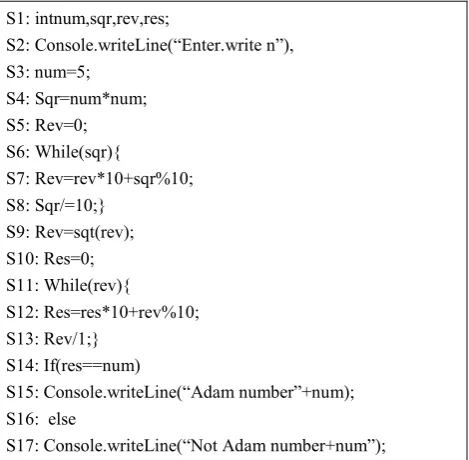
Consider an example of C#.net program and its diagnosis matrix in Table1 to see how to use the test information and how to locate the suspicious statement in the following sections.

S1: intnum,sqr,rev,res;

S2: Console.writeLine(“Enter.write n”), S3: num=5;

S4: Sqr=num*num; S5: Rev=0; S6: While(sqr){

S7: Rev=rev*10+sqr%10; S8: Sqr/=10;}

S9: Rev=sqt(rev); S10: Res=0; S11: While(rev){

S12: Res=res*10+rev%10; S13: Rev/1;}

S14: If(res==num)

S15: Console.writeLine(“Adam number”+num); S16: else

S17: Console.writeLine(“Not Adam number+num”);

Fig. 1 Sample C# .net program

The program in Fig. 1 is to check the number is adam or not.

Table 1. Diagnosis matrix of program p

Statement No. T1(3) T2(5) T3(12) T4(15)

S1 1 1 1 1

S2 1 1 1 1

S3 1 1 1 1

S4 1 1 1 1

S5 1 1 1 1

S6 1 1 1 1

S7 1 1 1 1

S8 1 1 1 1

S9 1 1 1 1

S10 1 1 1 1

S11 1 1 1 1

S12 1 1 1 1

S13 1 1 1 0

S14 1 1 1 0

S15 1 0 1 0

S16 0 1 0 0

S17 0 1 0 0

Table 1 shows the test cases in T and its corresponding execution path. The program produces correct outputs on all testcases except T4, in Table 1. Because s11 uses the expression Rev%1 instead of Rev%10for testcaseT4

4. PROBABILISTIC BASED APPROACH

In this section, we discuss the two models that form the basis for the Probabilistic Program Dependence Graph. The first is the program dependence graph, which represents structural dependences between program statements. The second is a dependency network, which is a type of probabilistic graphical model that represents conditional dependence and independence relationships between random variables.

Definition 1:

A Dependency Network[18] is a triple (S,G,Ω), where S represents a set of random variables, G=(N,E) is a possibly cyclic directed graph, and Ω represents a set of conditional probability distributions. N and E are the set of nodes and set of directed edges in G respectively, with nodes in G corresponding to random variables in S and edges in G representing dependences among the random variables

Definition 2:

fact Definition 3:

A program dependence graph (PDG)[18] is a directed graph whose nodes represent program statements and whose edges represent data and control dependences. Lables on the control dependence edges represent the truth values of the branch conditions for those edges, and labels on data dependence edges represent the variables whose values flow along those edges.

Definition 4:

A probabilistic program dependence graph (PPDG)[18] for program P is a tripe (G,S,Q),where G=(N,E) is the transformed PDG of P whose nodes and edges sets are N and E, respectively, and S and Q are mapping from nodes to states and from nodes to conditional probability distributions, respectively.

Fig. 2: Steps in the construction of a PPDG.

In this paper we show how the PPDG can be used for fault localization .Given a program P it generates the PDG and then transforming it into PPDG by adding nodes and edges to it and specifies the states of the nodes we call the graph that results after transforming the PDG termed as transformed PDG.

Steps for generating PPDG:

Step 1: Generates the PDG for given input program.

Step 2: Transforming the PDG by adding nodes and edges and also specifying the states of the nodes.

Step 3: It inserts probes into program P to find execution data require to estimate the parameters of the PPDG and produce the instrumented program p’.

Step 4: In this step we generate the execution data by combining p’ with test suit Tp.

Step 5: The learning step generates a PPDG based on the execution data and the transformed PDG.

Using System;

1 Class fact

2 {

3 Int f=1; int n=5; int i=0;

4 While(i<n)

5 {

6 f=f*i; i++;

7 Console.writeLine(f);

}

}

Fig. 3 Sample C# .Net program

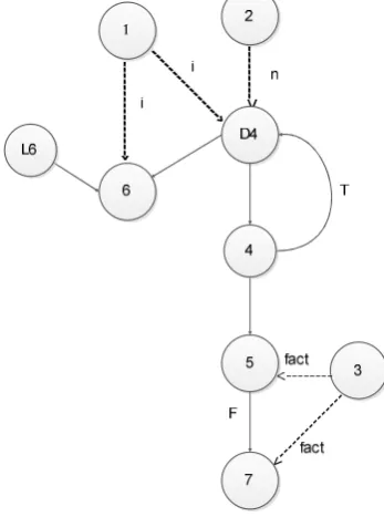
Fig. 3 Shows the program for find the factorial of a given number. Fig. 4 shows the control flow graph for given program. Node 1 represents the first statement in the program and node 6 represents the last statement in the program For example node 4 has two outgoing edges edge (4,5) is taken if the condition is true and edge (4,7) is taken if the condition 7 is false. Using the control flow graph, we can define both control dependence and data dependence.

Fig. 4 Control Flow Graph

From the control flow graph the PDG is generated as shown in Fig. 5. The PDG is generated with the combination of control flow graph and dataflow graph The nodes in the PDG represent line numbers of corresponding statements in the program. Solid edges represent control dependences and dotted edges represent data dependences between nodes. If the edges represents control dependences then it is labiled with T or F. if the edges represents data dependence then it is labeled by variable name.

PDG transformation

In this step PDG is transformed structure by adding nodes and edges to it and specify the states of the node then it is called as transformed PDG.

--->

--- ---

---_->

Fig. 6 Transformed PDG

Structural Transformation

In this transformation adds nodes and edges in two cases.

i) If a node has 2 state component(i.e predicate and data dependence component)

ii) If a node has self loops (i.e nodes have control or data dependences on themselves in the PDG.

For example the predicate “i<n” at node 4 has two state components because of the predicate computation at the node 4 because of its dynamic data dependences on nodes 3 and 6. Fig. 6 shows the results of the structural transformation of the PDG of fact that introduces new nodes D4. A self-loop in a PDG may involve either a control dependence or a data dependence. If a node n is data dependent on itself with respect to a program variable v, our technique removes the self-loop and adds a new node. The new node is an immediate predecessor of n. The edge from the new node to n is a data dependence edge with respect to variable v. For example, in Fig. 5, node 6 is data dependent on itself. The self-loop is removed and a new node L6 is introduced. L6 is the immediate predecessor of node 6 (i.e., node 6 becomes data dependent on L6 with the data dependence variable being i). Fig. 6 shows the result of the self-loop transformation.

State Specification

This technique models the states of each node after finding the transformed PDG of sample program.

Predicate nodes

For example, Fig. 5 represents a predicate “i<n” at node 4. If n=5 and i=1 when node 4 is executed the predicate outcome is <. In general, our technique assigns <, >, = = and as the set of states to each predicate node whose operands are primitive variables. Laski and Korel [17] proposed that the states of non predicate nodes are dynamically data dependant on other nodes. It provides the data environment of statement s that reaches s along any paths and is used at s consider our example in Fig. 5, suppose that di(x) denotes a definition of a

variable x at node i. For node7, the data environment is {d3(fact), d5(fact)} because the definitions of “fact ”at nodes 3and 5 are potentially used at node 7.The elementary data contexts of node 7 are {d3(fact)}and{d5(fact)} because only one of the definitions can reach node 7at a time in an execution. The data context, is the set of its elementary data contexts, is {d3 (fact)} and {d5(fact)}. For node D4, the data environment and data context are (d1(i), d2(n)), (d6(i), d2(n))

respectively. The data contexts of nodes D4, 6, and 7 are (d1(i)), (dl6(i)), (d3(fact)), (d5(fact)), respectively.

5. LEARNING

This technique finds the parameters of PPDG using set of execution data ₍

{ }

0

n k k

D

D= = generated by P with its test suite Tp. In this technique uses node state trace information to find the parameters of the PPDG.A node state trace is a set of executed nodes which are active in transformed PDG. For each Dk∈D is a node state trace. A node can be multiple times

in the trace so that states of node can also be different. We used batch learning algorithm for finding the parameters

The parameters of the PPDG are estimated by conditional probability table(CPTs). Conditional probability distributions are represented by tables because the nodes in transformed PDG are discrete. Suppose that X={X1,….,Xn} represents the set of nodes in the transformed PDG.

For a node with no parents our technique estimates the probabilities (P(xj=xji)) of the nodes as

) (

) ( ) (

j jj j ji j

X n

x X n x X

p = = =

Where n(Xj=xji) is the number of times nodes (Xj) in

state xji across all node state traces and n(xj) is the number of

times the node Xj occurs across all node state traces.

Table 2 Nodes in Transformed PDG with Corresponding States

Nodes states

1,2,3,L6

D4

4

5

6

7

T,

(d1(i),d2(n)),(d6(i),d2(n))

>,<,==,

(d3(fact)),(d1(i)),

(d1(i)),(dl6(i)),

Table 3. Nodes in Transformed PDG with Corresponding Conditional Probability Distributions

Nodes Conditional Probability Distribution

1,2,3,L6 D4 4 5 6 7 P(1),P(2),P(3),and P(L6) P(D4|1,2,6) P(4|D4) P(5|1,3,4) P(6|1,4,L6) P(7|3,5)

For a node with parents our technique estimates the probabilities (p(Xj=xji|pa(Xj) =pa ji))of the node as

), Pa ) X ( Pa ( n ) Pa ) X ( Pa . x X ( n pa = ) Pa(X | x = p(X ji j ji j ji j ji j ji j ₌ = = = (3)

Where n(Xj=xji. Pa(Xj)=Paji) is the number of times

node Xj and its parents assume a specific state configuration

allows all node state traces. A state configuration in a set of states assigned to a set of nodes in the PPDG. The CPTs of the nodes is the sum over the states of node Xj given that its

parents are in a specific state configuration paji must

equal 1.0. 0 . 1 ) pa ) X ( Pa ( | s x ( P ji x x s j j ji ji = = =

∑

Algorithm: Learmparam

Input: D = ; transformed PDG

Output: PPDG

1 foreachDk€ D do

2 for j=1 to length(Dk) do

3 if Pa(Xj)=0 then

4 Increment n(Xj = xji) by 1, where xji is then Current

state of Xj

5 else

6 Increment n(Xj = xji.Pa(Xj) = paji) by 1,where Xji is

the current state conFig.uration of the parents of Xj

7 end

8 end

9 end

10 Compute probabilities of Xj using equation (5), (2)

return PPDG

Fig.7 Batch Learning Algorithm

The input to the algorithm is a set of execution data with its test suite Tp and transformed PDG then the output is PPDG. Different types of execution data ( coverage and trace information)are used to estimate the parameters of the PPDG.

A node state trace in a set of executed nodes in the transformed PDG. It is uses node state to estimate the parameters of the PPDG. As it process from beginning to end of each Di∈D changing the state of the parents and increase the probability.

For node with parents it computes the conditional probability of present node. For node without parents it computes the conditional probability and it increments the probability of current node. For the above example using the learnparameter algorithm probability is calculated. The probability for each node is calculated and given in Table 4.

Table 4. Conditional probability distribution

Node Probability

1 1

2 1

3 1

4 1.0

5 0.5

6 0.4

7 0.2

6 FAULT LOCALIZATION

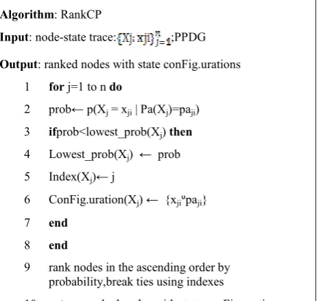
Software debugging is one of the difficult task in software. For finding the fault several fault localization technique are available. In this paper RankCPalogorithm [18] is used for finding the fault. It examines a single failing execution at a time. It ranks the nodes based on conditional probability of nodes having parents. RankCPalgorithm finds the first causes of a failure of a node Xj given the state of its parents.

Algorithm: RankCP

Input: node-state trace: ;PPDG

Output: ranked nodes with state conFig.urations

1 for j=1 to n do

2 prob← p(Xj = xji | Pa(Xj)=paji)

3 ifprob<lowest_prob(Xj) then

4 Lowest_prob(Xj) ← prob

5 Index(Xj)← j

6 ConFig.uration(Xj) ← {xjiᶸpaji}

7 end

8 end

9 rank nodes in the ascending order by probability,break ties using indexes

10 return ranked nodes with state conFig.urations

Fig. 8 RankCP Algorithm

probability for the current node (xji) and its parent node Paji

(ie.,P(Xji|Pa(Xj)=Paji)). For each node Xj it finds the lowest

probability using the conditional probability table .if a node has same probability value then it ranks the node with lowest index value.

7. EXPERIMENTS

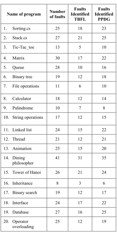
In our experiments we evaluate the effectiveness of fault detection techniques by finding the fault detection rate .We considered 20 c#.Net programs. We have generated PPDG for the programs. Fault Localization is carried out by TBFL and PPDG. For evaluation purpose we have included faults randomly into our input test cases. Table 5 shows the results of both the Fault localization technique for different C#.Net programs.

Table. 5 Faults identified by TBFL and PPDG

Name of program Number of faults

Faults Identified

TBFL

Faults Identified

PPDG

1. Sorting.cs 25 18 23

2. Stack.cs 27 21 25

3. Tic-Tac_toe 13 5 10

4. Matrix 30 17 22

5. Queue 28 10 16

6. Binary tree 19 12 18

7. File operations 11 6 10

8. Calculator 18 12 14

9. Palindrome 10 7 8

10. String operations 17 12 15

11. Linked list 24 15 22

12. Thread 21 12 21

13. Animation 25 15 20

14. Dining philosopher

41 31 35

15. Tower of Hanoi 26 21 24

16. Inheritance 8 3 6

17. Binary search 19 12 17

18. Interface 24 17 22

19. Database 27 16 25

20. Operator overloading

25 12 19

From the results we are noticed that our proposed method has more fault localization rate than TBFL method.

Fig. 9 Comparison between TBFL and PPDG

The performance analysis measure is shown in the Fig. 9. Consider for example the. Net Program sorting. In this program number of faults identify by TBFL is 18. But for same program PPDG identifies 23 faults thus we can conclude that PPDG is efficient than TBFL.

8. CONCLUSION AND FUTURE WORK

In this paper we developed an fault localization technique based on statistical dependences between program elements. Here we used RankCP algorithm for finding the fault in the program. RankCP algorithm uses the conditional probability from PPDG to rank the nodes from most suspicious to least suspicious. In existing work fault localization in done for object oriented programming language such as c,c++ and java. In the proposed work fault localization is applied for Dotnet programs. Learnparam approach is used to estimate the parameters of PPDG from the set of executed data. We used RankCP algorithm for fault localization of PPDG.PPDG is generated based on the execution data and transformed PDG. We compared two fault localization techniques such as TBFL and PPDG and the result shows that PPDG is effective model for representing program behaviours particularly that associated with faults. This work may be extended to find memory related faults.

9. REFERENCES

[1] FeiPu, Yan Zhang, Localizing Program Errors Via slicing Reasoning. IEEE High Assurance systems Engineering symposium, 187-196, 2008.

[2] Damiano Zanardini, The semantics of program slicing

,IEEE 2008

[3] T. Gyimothy , A. BESzedes, and I.Forgacs. An efficient relevant slicing method for debugging. In symposium on Foundations of Software Engineering (FSE’99), 303-321, ACM, 1999.

[4] Sun Ji-Rong, Ni Jian-cheng, and Li Bao-Lin. Dichotomy method in testing –based fault localization. International Journal of Mathematical models and methods in applied sciences,2007.

[5] M. Renieris and S. P. Reiss, “Fault Localization with Nearest Neighbor Queries,” In Proceedings of the 18th IEEE International Conference on Automated Software Engineering, pp. 30-39, Montreal, Canada, October 2003.

[7] B. Liblit, M. Naik, A. X. Zheng, A. Aiken, and M. I. Jordan, “Scalable Statistical Bug Isolation,” in Proceedings of the 2005 ACM SIGPLAN Conference on Programming Language Design and Implementation, pp. 15-26, Chicago, Illinois, USA, June, 2005.

[8] W. Eric Wong, Program Debugging with Effective Software Fault Localization IEEE Transactions on Reliability 61(1): 149-169 (2012).

[9] W. E. Wong, T. Wei, Y. Qi, and L. Zhao, “A Crosstab-based Statistical Method for Effective Fault Localization,” in Proceedings of the 1st International Conference on Software Testing, Verification and Validation, pp. 42-51, Lillehammer, Norway, April 2008. [10]Zeller, “Isolating Cause-Effect Chains from Computer Programs,” in Proceedings of the 10th ACM SIGSOFT Symposium on Foundations of Software Engineering, pp. 1-10, Charleston, South Carolina, USA, November 2002.

[11]T. Zimmermann and A. Zeller, “Visualizing Memory Graphs,” in Proceedings of the International Seminar on Software Visualization, pp. 191-204, Dagstuhl Castle, Germany, May 2001.

[12]N. Gupta, H. He, X. Zhang, and R. Gupta, “Locating Faulty Code Using Failure-Inducing Chops,” in Proceedings of the 20th IEEE/ACM International Conference on Automated Software Engineering, pp. 263-272, Long Beach, California, USA, November 2005.

[13]Y. Brun and M. D. Ernst, “Finding Latent Code Errors via Machine Learning over Program Executions”, in Proceedings of the 26th International Conference on Software Engineering, pp. 480- 490, Edinburgh, UK, May 2004.

[14]Eric Wong, Vidrohadebroy, “Software fault localization” W. IEEE Annual Technology Report, 2009.

[15]M.Weiser. Program slicing. IEEE transactions on software engineering, SE-10(4):352-357, 1984

[16]J.W. Laski and B. Korel, “A Data Flow Oriented Program Testing Strategy,” IEEE Trans. Software Eng., vol. 9, no. 3, pp. 347-354, May1983.