How to cite this paper:Mohamed, A. and Peng, Q.Y.(2014) Particle Swarm Optimization (PSO) Performance in Solving the Train Location Problem at Transshipment Yard. Open Access Library Journal, 1: e1024.
http://dx.doi.org/10.4236/oalib.1101024
Particle Swarm Optimization (PSO)
Performance in Solving the Train Location
Problem at Transshipment Yard
Alhossein Mohamed, Qiyuan Peng
School of Transportation and Logistics, Southwest Jiaotong University, Chengdu, China Email: [email protected]
Received 20 July 2014; revised 2 September 2014; accepted 6 October 2014
Copyright © 2014 by authors and OALib.
This work is licensed under the Creative Commons Attribution International License (CC BY).
http://creativecommons.org/licenses/by/4.0/
Abstract
Particle swarm optimization (PSO) is an evolutionary computation technique; it has shown its ef-fectiveness as an efficient, fast and simple method of optimization. In this paper, the mathematical model represents NP-hard in the strong sense; since any instance of the quadratic assignment problem (QAP), I will implement the particle swarm optimization (PSO) for the quadratic assign-ment problem (QAP). The results show that the PSO is an appropriate optimization tool for use in determining the train location in the transshipment yard by comparing it with previous studies to know the PSO’s performance.
Keywords
Particle Swarm Optimization, Transshipment Yards, Train Location
Subject Areas: High Performance Computing, Information and Communication Theory and Algorithms
1. Introduction
OALibJ | DOI:10.4236/oalib.1101024 2 October 2014 | Volume 1 | e1024
transshipment and detailed results are shown and compared with other evolutionary algorithms results.
2. Problem Description
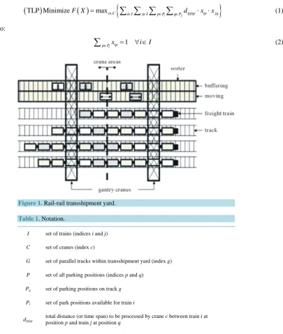
The train location problem (TLP) has to be solved perpetually for every pulse of trains arriving at a transship-ment yard. The TLP assigns each train of the given pulse a track (vertical parking position) and additionally de-cides on each train’s horizontal parking position along the yard. It is the aim of the TLP to evenly spread the overall workload among the given gantry cranes of the yard, so that by minimizing the maximum workload of cranes train processing of a given pulse is accelerated. This basic decision problem relies on some premises [1].
With suited parameters dipjqc on hand and the additional notation summarized in Table 1 the train location
problem (TLP) can be formalized by a quadratic program consisting of objective function (1) subject to con-straints (2) to (4):
(
TLP Minimize max)
( )
{
}
i j
c C i I j I p P q P ipjqc ip jq
F X = ∈
∑ ∑ ∑ ∑
∈ ∈ ∈ ∈ d ⋅x ⋅x (1)Subject to:
1
i ip
p P∈ x = ∀ ∈i I
[image:2.595.132.538.226.705.2]∑
(2) [image:2.595.150.490.236.514.2]Figure 1. Rail-rail transshipment yard.
Table 1. Notation.
I set of trains (indices i and j)
C set of cranes (index c)
G set of parallel tracks within transshipment yard (index g)
P set of all parking positions (indices p and q)
Pg set of parking positions on track g
Pi set of park positions available for train i
dipjqc total distance (or time span) to be processed by crane c between train i at position p and train j at position q
OALibJ | DOI:10.4236/oalib.1101024 3 October 2014 | Volume 1 | e1024
1
q ip
i I∈ p P∈ x = ∀ ∈g G
∑ ∑
(3){ }
0,1 ,ip i
x ∈ ∀ ∈i I p∈P (4) In objective function (1) the maximum workload of all cranes c∈C is to be minimized, where each crane’s workload is determined by summing up the respective workload parameters dipjqc whenever train i is parked on
position p (with xip= 1) and another train j is parked on position q (with xjq = 1). Equalities (2) ensure that each
train i of the given pulse I is assigned to exactly one parking position out of its possible positions Pi. On the
oth-er hand, it is to be ensured (constraints (3)) that each track g receives exactly one train, where Pg ⊂P com-prises all parking positions of track g. Finally, binary variables xip are defined by (4).
Obviously, TLP with facultative weights dipjqc is NP-hard in the strong sense, since any instance of the
qua-dratic assignment problem (QAP) can be easily reduced to an instance of TLP with a single crane C=
{ }
1where the length of all trains is equal to the length of the yard, so that only one parking position per track is feasible. QAP was proven to be NP-hard in the strong sense by Sahni and Gonzalez (1976).
This problem had been studies by Michael Kellner, Nils Boysen, Malte Fliedner [1] using efficient heuristic solution procedures to solve it, which they used a myopic heuristic procedure and two meta-heuristics, a simu-lated annealing approach and a genetic algorithm. And today I am going to solve it by particle swarm optimiza-tion (PSO). Appling the particle swarm optimizaoptimiza-tion tools in mat lab programming software.
3. Particle Swarm Optimization Implementation
3.1. Particle Swarm Model
The classical PSO model consists of a swarm of particles, which are initialized with a population of random candidate solutions. They move iteratively through the d-dimension problem space to search the new solutions, where the fitness, f, can be calculated as the certain qualities measure [2]. Each particle has a position represented by a position-vector xi(i is the index of the particle), and a velocity represented by a velocity-vector
vi. Each particle remembers its own best position so far in a vector xi#, and its j-th dimensional value is
#
ij
x . The best position-vector among the swarm so far is then stored in a vector x*, and its j-th dimensional value is
j
x∗. During the iteration time t, the update of the velocity from the previous velocity to the new velocity is de-termined by Equation (5). The new position is then dede-termined by the sum of the previous position and the new velocity by Equation (6).
( )
(
)
(
#(
)
(
)
)
(
(
)
(
)
)
1 1 2 2
1 1 1 1 1
ij ij ij ij j ij
v t =wv t− +c r x t− −x t− +c r x t∗ − −x t− (5)
( )
(
1)
( )
ij ij ij
x t =x t− +v t (6) where r1 and r2 are the random numbers in the interval [0, 1]. c1 is a positive constant, called as coefficient of the self-recognition component, c2 is a positive constant, called as coefficient of the social component. The variable
w is called as the inertia factor, which value is typically setup to vary linearly from 1 to near 0 during the iterated processing. From Equation (5), a particle decides where to move next, considering its own experience, which is the memory of its best past position, and the experience of its most successful particle in the swarm.
In the PSO model, the particle searches the solutions in the problem space within a range
[
−s s;]
(if the range is not symmetrical, it can be translated to the corresponding symmetrical range). In order to guide the par-ticles effectively in the search space, the maximum moving distance during one iteration is clamped in between the maximum velocity[
−vmax;vmax]
given in Equation (7), and similarly for its moving range given in Equation (8):( )
(
)
, sign , min , , max
i j i j i j
v = v v v (7)
( )
(
)
, sign , min , , max
i j i j i j
OALibJ | DOI:10.4236/oalib.1101024 4 October 2014 | Volume 1 | e1024 Algorithm: Particle Swarm Optimization Algorithm
01. Initialize the size of the particle swarm n, and other parameters. 02. Initialize the positions and the velocities for all the particles randomly. 03. While (the end criterion is not met) do
04. t= +t 1
05. Calculate the fitness value of each particle;
06. arg min1
(
(
( 1 ,))
(
1( ))
,(
2( ))
, ,(
( ))
, ,(
( ))
)
n
i i n
x∗= = f x t∗ − f x t f x t f x t f x t
07. For i = 1 to n
08. #( )
(
(
#( ))
(
( ))
)
1arg minn 1 ,
i i i i
x t = = f x t− f x t ;
09. For j = 1 to d
10. Update the j-th dimension value of xi and vi 10. according to Eqs.
12. Next j 13. Next i 14. End While.
3.2. Experiment Settings
3.2.1. Yard Layout
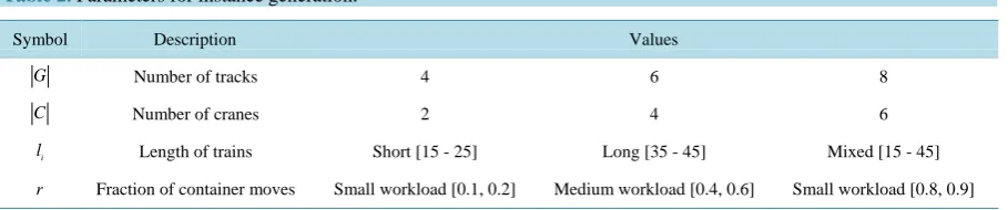
With regard to the yard layout, we base the study on the typical setting of German transshipment yards. A typi-cal yard length is 700 meters and slots are adjusted to accommodate standard railcars with a total length of 14 meters. Thus, we assume a yard length of T = 50 slots, with a horizontal distance of dh = 14 meters between any two adjacent slots. Furthermore, we assume a vertical distance of dv = 7 meters between neighboring tracks and the sorter, which is located below the final track. The number G of parallel tracks and the number C of gantry cranes are varied as follows: G∈
{
4, 6,8}
and C∈{
2, 4, 6}
, so that differently sized transshipment yards are investigated.3.2.2. Container Moves
The train length (in slots) is randomly determined, where different scenarios (short trains only, long trains only and mixed train lengths) are generated by drawing liout of intervals [15 - 25], [35 - 45] and [15 - 45],
respec-tively. Furthermore, we aim to investigate different workload settings, namely low, medium and high workload. Therefore, γ = ⋅r Mmax container moves are determined by randomly drawing trains i and j and train posi-tions k and l (counted from the engine) for each move, where i≠ j must hold. Mmax and r denote the maxi-mum number of container moves (for given train lengths) and a fraction value randomly drawn from intervals [0.1, 0.2] (low), [0.4, 0.6] (medium) and [0.8, 0.9] (high workload), respectively.
3.2.3. Technical Crane Parameters
The gantry cranes move in horizontal and vertical direction simultaneously driven by independent engines. In horizontal direction the whole crane moves on special rail tracks, whereas vertically merely the steeple cab car-rying the spreader is moved. Thus, the maximum time span for executing the vertical and horizontal movement determines the processing time of a container move. We assume a velocity of crane and steeple cab of ve = 3 meters per second, if the crane moves empty, whereas the velocity reduces to vl = 2 meters per second, if a con-tainer is carried. Once positioned, picking and dropping of concon-tainers requires additional processing time. Espe-cially, locating the spreader is precision work, so that we assume a typical time span of td = 45 seconds for pick-ing or dropppick-ing a container. See Alicke (2002) and Martinez et al. (2004) for comparable parameters.
3.2.4. Crane Movement
A typical real-world policy to determine the division of labor among cranes is to partition the yard into equally sized areas (Boysen and Fliedner, 2009). Thus, we follow this widespread approach and assign each given crane the same number of slots (accounting for rounding differences). If a bundle of trains is parked and, thus, all con-tainer moves are fixed and assigned to gantry cranes, sequencing moves per crane remains a complex optimiza-tion problem.
OALibJ | DOI:10.4236/oalib.1101024 5 October 2014 | Volume 1 | e1024
However, the sequence of container moves is typically not optimized by a scheduling procedure but locally determined by the respective crane operator. Thus, to simulate a human decision rule we apply a simple nearest neighbor heuristic. Each crane’s starting position is the left hand border of its area, while the steeple cab is posi-tioned over the sorter. From there it consecutively executes the container move closest to its current position. Split moves, e.g., from yard area A to B, are considered by updating crane B’s list of unprocessed container moves, not before the respective container arrived in the sorter-segment of crane B. Thus, the list is updated just after crane A processed the first part of the split move (from train into the sorter) and a vehicle (with sorter ve-locity vs = 3) moved the container into yard area B. With regard to the sorting system it is assumed that vehicles are not a bottleneck and congestions do not occur.
The aforementioned parameters of instance generation are summarized inTable 2. All parameters are com-bined in a full-factorial design and for each parameter constellation 10 replications are generated, so that 3 × 3 × 3 × 3 × 10 = 810 different instances were obtained.
For each of these instances a preprocessing has to be executed, which determines weights dijklc of total
work-load resulting from work-loaded moves for each train pair i and j and feasible parking positions of trains. If feasible positions of a train pair are presumed, the workload wD of a direct container move from track t and slot s to track
t' and slot s' can be determined as follows:
( ) (
)
(
, , ,)
2 max ;h v
D p
l l
s s d t t d w t s t s t
v v − ⋅′ − ⋅′ ′ ′ = ⋅ +
If processed as a direct move, a container move
(
( ) (
t s, , t s′ ′,)
)
requires a pick and a drop operation( )
2⋅tp . Additionally, the time for the actual move is to be added, which amounts to the maximum of the crane’s hori-zontal and vertical distance each weighted with velocity vl (for a loaded move). Split moves into (with weightwIN) and out of (with weight wOUT) the sorter also require a pick and drop operation and the actual movement time, which is required for the vertical movement between rail track and sorter track ts:
( ) ( )
(
)
(
)
(
) (
)
(
)
(
)
IN OUT, , , 2
, , , 2
v s p s l v s p s l
t t d
w t s t s t
v
t t d
w t s t s t
v − ⋅ = ⋅ + ′ − ⋅ ′ ′ ′ = ⋅ +
The sum of resulting workload weights w for the respective container moves between two trains amount to weights dijklc. Note that the workload of empty moves required for the yard simulation can be calculated in the
same fashion. Then, the four heuristic solution procedures are applied to determine parking positions of trains. First, with regard to the solution performance these results are compared to optimal TLP objective values, so that the gap of our heuristic procedures can be determined. Then, resulting parking positions of trains are passed over to our yard simulation, where the schedules of cranes and sorter are determined. This way, the workload of loaded moves (as considered in model TLP) can be compared to the real-world workload (approximated by the simulation), so that the suitability of our surrogate objective and the acceleration of container processing ob-tained by optimized parking positions can be determined.
3.3. Yard Simulation
[image:5.595.88.543.627.722.2]The results of our yard simulation, Here, parking positions of trains obtained by TLP are passed over and real- world crane and sorter operations are simulated. This way, the results of TLP can be compared with the resulting
Table 2. Parameters for instance generation.
Symbol Description Values
G Number of tracks 4 6 8
C Number of cranes 2 4 6
i
l Length of trains Short [15 - 25] Long [35 - 45] Mixed [15 - 45]
OALibJ | DOI:10.4236/oalib.1101024 6 October 2014 | Volume 1 | e1024
(approximate) real-world workload of cranes. While TLP minimizes the cranes’ workload merely on the basis of loaded moves (surrogate objective, denoted as SURR), the yard simulation provides the actual workload con-sisting of loaded and empty crane moves (actual objective, denoted as ACT). On average over all 810 instances, the workload of SURR determined by our best-performing PSO procedure already makes up 89.01% of the val-ue of ACT, which results from the over proportional inflval-uence of time consuming pick and drop operations. Moreover, the coefficient of correlation (Pearson’s product-moment correlation) between both approaches amounts to a remarkable 0.9992. Thus, the conclusion can be drawn, that our surrogate objective of merely con-sidering loaded moves is a suited simplification. On the one hand, the actual objective of reducing the overall workload is strongly supported and, on the other hand, the solution process is considerably alleviated by ex-cluding a detailed crane scheduling.
Furthermore, we aim at investigating the question whether optimized parking positions enable a considerable reduction of train processing time compared to real-world policy RWP. Recall that RWP assigns tracks accord-ing to a first-come-first-serve policy and parks all trains in slot 1. As performance measures, we report the aver-age absolute deviation (labeled avg abs) between both policies with regard to the makespan of processing the current bundle of trains as approximated by our simulation study. Avg abs denominates the acceleration of train processing if improved parking positions are applied instead of RWP in minutes averaged over all instances of the respective parameter constellation. Furthermore, the average relative deviation (labeled avg rel) of both pol- icies in percent is reported, where the deviation is measured by
(
)
( )
( )
RWP
100
F F
F
δ δ
−
∗ with F
(
RWP)
and( )
[image:6.595.87.538.369.716.2]F δ being the make span of our yard simulation when parking positions are determined by a real-world rule of thumb or improved with one of our heuristic procedures δ∈
{
MSP,SA, GA, PSO}
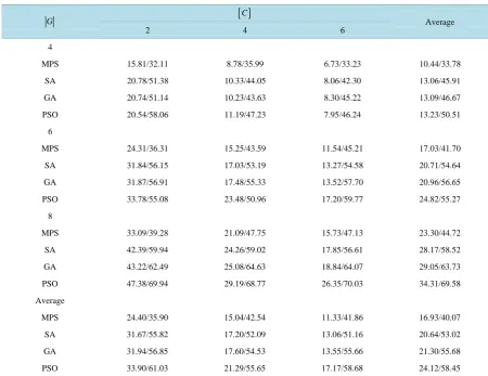
respectively. Table 3Table 3. Absolute and relative speed-up of container processing time depending on yard size.
G [ ]C Average
2 4 6
4
MPS 15.81/32.11 8.78/35.99 6.73/33.23 10.44/33.78
SA 20.78/51.38 10.33/44.05 8.06/42.30 13.06/45.91
GA 20.74/51.14 10.23/43.63 8.30/45.22 13.09/46.67
PSO 20.54/58.06 11.19/47.23 7.95/46.24 13.23/50.51
6
MPS 24.31/36.31 15.25/43.59 11.54/45.21 17.03/41.70
SA 31.84/56.15 17.03/53.19 13.27/54.58 20.71/54.64
GA 31.87/56.91 17.48/55.33 13.52/57.70 20.96/56.65
PSO 33.78/55.08 23.48/50.96 17.20/59.77 24.82/55.27
8
MPS 33.09/39.28 21.09/47.75 15.73/47.13 23.30/44.72
SA 42.39/59.94 24.26/59.02 17.85/56.61 28.17/58.52
GA 43.22/62.49 25.08/64.63 18.84/64.07 29.05/63.73
PSO 47.38/69.94 29.19/68.77 26.35/70.03 34.31/69.58
Average
MPS 24.40/35.90 15.04/42.54 11.33/41.86 16.93/40.07
SA 31.67/55.82 17.20/52.09 13.06/51.16 20.64/53.02
GA 31.94/56.85 17.60/54.53 13.55/55.66 21.30/55.68
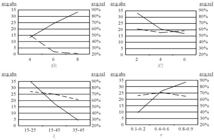
OALibJ | DOI:10.4236/oalib.1101024 7 October 2014 | Volume 1 | e1024 Figure 2. Absolute and relative speed-up in dependency of parameters of instance generation.
lists both performance measures in dependency of the parameters: number G of tracks and number C of cranes, which together reflect the size of a transshipment yard. The results reveal a remarkable potential for ac-celerating train processing. Depending on the size of the yard, possible absolute accelerations (avg abs) of our best-performing PSO procedure deviate between 47.38 minutes with eight tracks (high overall workload) and two cranes (low division of labor) and 7.95 minutes with four tracks (low overall workload) and six cranes (high division of labor). Interestingly, the relative acceleration (avg rel) of train processing performs somewhat con-trarily. This is explained by the fact, that with a high division of labor the average make span tends to be lower in value, because a pulse of trains is processed much faster.
As a consequence a comparable absolute reduction in makespan leads to a higher relative reduction. In rela-tive terms, train processing is accelerated by between 47.23% and 70.03% whenever parking positions are de-termined by PSO.
Further conclusions (in terms of a sensitivity analysis) can be drawn if the speed-up of improved parking po-sitions (determined with PSO) is related to the parameters of instance generation. Therefore,Figure 2 displays the average relative deviation (avg rel in %) and the average absolute deviation (avg abs in minutes) in depen-dency of the parameters: number G of tracks, number C of cranes, interval of train lengths li and interval
of fraction value r, which determines the number of containers (workload) to be processed, respectively.
4. Conclusions
• With an increasing number G of tracks the overall workload is increased.
• The higher the division of labor (more cranes C ), the lower the absolute (avg abs) speed-ups of optimal parking positions, whereas relative speed-up remains almost unaffected by additional cranes.
• With shorter trains more degrees of freedom exist with regard to finding feasible parking positions within a yard.
• With an increasing fraction of value r,the number of containers transshipped rises.
The performance of particle swarm optimization (PSO) method was studied in this paper compared with tra-ditional and other evolutionary optimization methods and gave the best results in solving the problem.
References
Frie-OALibJ | DOI:10.4236/oalib.1101024 8 October 2014 | Volume 1 | e1024 drich-Schiller-Universität Jena, Lehrstuhl für Operations Management, Germany.