Quantum Inspired Particle Swarm Optimization Algorithm Encoded by Probability Amplitudes of Multi Qubits

http://dx.doi.org/10.4236/ojop.2015.42003

Quantum-Inspired Particle Swarm

Optimization Algorithm Encoded by

Probability Amplitudes of Multi-Qubits

Xin Li1, Huangfu Xu2, Xuezhong Guan2

1_{School of Computer and Information Technology, Northeast Petroleum University, Daqing, China}

2_{School of Electrical and Information Engineering, Northeast Petroleum University, Daqing, China}

Email: lixin_dq@163.com

Received 9 February 2015; accepted 12 May 2015; published 14 May 2015

Copyright © 2015 by authors and Scientific Research Publishing Inc.

This work is licensed under the Creative Commons Attribution International License (CC BY).

http://creativecommons.org/licenses/by/4.0/

Abstract

To enhance the optimization ability of particle swarm algorithm, a novel quantum-inspired par-ticle swarm optimization algorithm is proposed. In this method, the parpar-ticles are encoded by the probability amplitudes of the basic states of the multi-qubits system. The rotation angles of mul-ti-qubits are determined based on the local optimum particle and the global optimal particle, and the multi-qubits rotation gates are employed to update the particles. At each of iteration, updating any qubit can lead to updating all probability amplitudes of the corresponding particle. The expe-rimental results of some benchmark functions optimization show that, although its single step itera-tion consumes long time, the optimizaitera-tion ability of the proposed method is significantly higher than other similar algorithms.

Keywords

Quantum Computing, Particle Swarm Optimization, Multi-Qubits Probability Amplitudes Encoding, Algorithm Design

1. Introduction

strate-gy [7]. These approaches enhance the PSO performance in different degrees. Quantum computing is an emerg-ing interdisciplinary, combinemerg-ing the information science and quantum mechanics, and its integration with intel-ligent optimization algorithms begun in the 1990s; there is quantum-behaved particle swarm optimization algo-rithm [8], quantum-inspired evolutionary algorithm [9], quantum-inspired harmony search algorithm [10], quantum-inspired immune algorithm [11], quantum-inspired genetic algorithm [12], and quantum-inspired de-rivative differential evolution algorithm [13]. In the algorithm mentioned above, Ref. [8] applied real-based code method; the other references employed single qubit probability amplitude to code individuals. In these kinds of coding, the adjustment of a qubit can only change one gene on the individual. However, in the multi-qubits probability amplitude-based code, with application of coherence quantum states, simply adjusting a qubit can change all probability amplitudes of the ground state in multi-bit quantum superposition states, and then update all genes on the individual. In this paper, we propose a new multi-qubits probability amplitude encoding-based quantum-inspired particle swarm optimization. Standard function extreme optimization experiments show the superiority of the proposed algorithm.

2. Basic PSO Model

There is M particles in the n-dimensional space. For the ith particle, its position Xi, velocity Vi, self-opti-

mum position L i

P , global optimum position Pg, are written as: Xi=

(

xi1,xi2,,xin

)

; Vi =

(

v vi1, i2,,vin

)

;

(

1, 2, ,

)

L

i = pi pi  pin

P ; Pg=

(

pg1,pg2,,pgn

)

. The update strategy of particles can be described as follows.

(

1

)

( )

1 1

(

( )

)

2 2

(

( )

)

L

i t+ =w i t +c r i − i t +c r g− i t

V V P X P X (1)

(

1

)

( )

( )

i t+ = i t + i t

X X V (2)

where i=1,,M , w is the inertia factor, c1 is itself factor, c2 global factor, r1, r2 is an uniformly

dis-tributed random number in (0, 1).

For convenience of description, Equation (1) can be rewritten as follows.

(

1

)

( )

[ ]

(

( )

)

i t+ =w i t + Φ i− i t

V V P X (3)

where

1 2

1 2

1 1

1 1 1 1

1 2 1 2 1 2 1 2

1 1 2 1 1 2 1 1 2 1 1 2

diag , , n L diag , , n

i i g

n n n n

c r c r

c r c r

c r c r c r c r c r c r c r c r

   

= _{ } + _{ }

+ + + +

     

P P P (4)

[ ]

(

1 2 1 2

)

1 1 2 1 1 2

diag c r c r , ,c rn c rn

Φ = +  + (5)

To make the PSO convergence, all particles must approximation Pi.

3. Multi-Bit Quantum System and the Multi-Bit Quantum Rotation Gate

3.1. Qubits and Single Qubit Rotation Gate

What is a qubit? Just as a classical bit has a state—either 0 or 1—a qubit also has a state. Two possible states for a qubit are the state 0 and 1 , which as you might guess correspond to the states 0 and 1 for a classical bit.

Notation like is called the Dirac notation, and we will see it often in the following paragraphs, as it is the standard notation for states in quantum mechanics. The difference between bits and qubits is that a qubit can be in a state other than 0 or 1 . It is also possible to form linear combinations of states, often called superposi-tion.

[

]

T

cos 0 sin 1 cos sin

φ = θ + θ = θ θ (6)

where θ is the phase of φ , cosθ and sinθ denote the probability amplitude of φ .

performing the quantum computation. A single qubit rotation gate can be defined as

( )

cos sin

sin cos θ θ θ θ θ ∆ − ∆   ∆ _{=  } ∆ ∆  

R (7)

Let the quantum state cos sin θ φ θ   =  

 , and φ can be transformed by

( )

(

)

(

)

cos sin θ θ θ θ θ  + ∆  ∆ _{=  } + ∆  

R . It is obvious

that R

( )

∆θ shifts the phase of φ .

3.2. The Tensor Product of Matrix

Let the matrix A has m low and n column, and the matrix B has p low and q column. The tensor product of A and B is defined as.

11 12 1

21 22 2

1 2

n

n

m m mn

A A A

A A A

A A A

      ⊗ =             

B B B

B B B

A B

B B B

(8)

where A_{i j,} is the element of matrix A.

3.3. Multi-Bit Quantum System and the Multi-Bit Quantum Rotation Gate

In general, for an n-qubits system, there are 2n of the form x x_{1 2}x_n ground states, similar to the single- qubit system, n-qubits system can also be in the a linear superposition state of 2n ground states, namely

[

]

1 2

1 2

1 1 1

T

1 2 1 2 00 0 00 1 11 1

0 0 _n n

n x x x n

x x x

a x x x a a a

φ φ φ

= =

=

∑ ∑ ∑

_ = _{  }

    (9)

where

1 2 n

x x x

a _ is called probability amplitude of the ground state x x1 2xn , and to meet the following

equa-tion.

1 2

1 2

1 1 1 ₂

0 0

1 n n

x x x

x x x

a

= =

=

∑ ∑ ∑

  (10)

Let φi =cosθi 0 +sinθi 1 , according to the principles of quantum computing, the φ φ1 2φn can be

written as

1 2

1 1 2

1 2 1 2

1

1 2

cos cos cos

cos

cos cos cos sin

sin sin

sin sin sin

n

n n

n n

n

n

θ θ θ

θ

θ θ θ θ

φ φ φ φ φ φ

θ θ

θ θ θ

        _{ } = ⊗ ⊗ =_{ }⊗ ⊗_{ }=      _{  }             (11)

It is clear from the above equations that, in an n-qubits system, any one of the ground state probability ampli-tude is a function ofn-qubits phase

(

θ θ1, 2,,θn

)

, in other words, the adjustment of any θi can update all 2

n

probability amplitudes.

In our works, the n-qubits rotation gate is employed to update the probability amplitudes. According to the principles of quantum computing, the tensor product of n single-qubit rotation gate R

( )

∆θi is n-qubits

rota-tion gate. Namely

(

∆ ∆θ θi 2 ∆θn

)

=

( )

∆θi ⊗

(

∆θ2

)

⊗ ⊗

(

∆θn

)

R  R R  R (12)

where

( )

cos sin

sin cos i i i i i θ θ θ θ θ ∆ − ∆   ∆ _{=  } ∆ ∆  

Taking n=2 as an example, the R

(

∆ ∆θ θ1 2

)

can be rewritten as follows.

(

)

1 2 1 2 1 2 1 2

1 2 1 2 1 2 1 2

1 2

1 2 1 2 1 2 1 2

1 2 1 2 1 2

cos cos cos sin sin cos sin sin

cos sin cos cos sin sin sin cos

sin cos sin sin cos cos cos sin

sin sin sin cos cos sin c

θ θ θ θ θ θ θ θ

θ θ θ θ θ θ θ θ

θ θ

θ θ θ θ θ θ θ θ

θ θ θ θ θ θ

∆ ∆ − ∆ ∆ − ∆ ∆ ∆ ∆ 

 _{∆ ∆ ∆ ∆ − ∆ ∆ ∆ ∆} 

∆ ∆ =

 ∆ ∆ − ∆ ∆ ∆ ∆ − ∆ ∆

 _{∆ ∆ ∆ ∆ ∆ ∆}

 R

1 2

os θcos θ      ∆ ∆ _

(13)

It is clear that

(

1 2

)

1 2 ˆ1 ˆ2 ˆ

n ∆ ∆θ θ ∆θ φ φn φn = φ ⊗φ ⊗ ⊗ φn

R (14)

where φˆi =cos

(

θi+ ∆θi

)

0 +sin

(

θi+ ∆θi

)

1 .

4. Particle Encoding Method Based on Multi-Bits Probability Amplitudes

In this paper, the particles are encoded by multi-qubits probability amplitudes. Let N denote the number of par-ticles, D denote the dimension of optimization space. Multi-qubits probability amplitudes encoding method can be described as follows.

4.1. The Number of Qubits Needed to Code

For an n-bits quantum system, there are 2n probability amplitudes, which can be used directly as a result of an individual encoding. In the D-dimensional optimization space, it is clear that _D≤2n

. Due to the constraint rela-tion between each probability amplitude (see to Equarela-tion (10)), hence _D<2n

. For the D-dimensional optimiza-tion problem, the required number of qubits can be calculated as follows.

( )

log 1

n= D + (15)

4.2. The Encoding Method Based on Multi-Qubits Probability Amplitudes First, generating randomly Nn-dimensional phase vector θi, i=1, 2,,N, as follows

[

1, 2, ,

]

i= θ θi i θin

θ (16)

where θij =2π rand× , rand is a random number uniformly distributed within the (0,1), j=1, 2,,n.

Let φij =cosθij 0 +sinθij 1 , using Equation (11), we can obtain following N n-qubits systems

11 12 1n

φ φ _φ , φ φ21 22φ2n , , φ φN1 N2φNn . In each of the quantum system, the first D probability

am-plitudes can be regarded as aD-dimensional particle code.

5. The Update Method Based on Multi-Qubits Probability Amplitudes

In this paper, the multi-bit quantum rotation gates are employed to update particles. Let the phase vector of the global optimal particle be θg = θ θg1, g2,,θgn, the phase vectors of the i

th

particle be θi=

[

θ θi1, i2,,θin

]

, and

the itself optimum the phase vector be 1, 2, ,

i i i bi = θ θb b θbn

θ .

From Equation (11), it is clear that, once θi has been updated, all its corresponding probability amplitudes

will be updated. To improve the search capability, in an iteration, all phases θi are updated in turn, which

al-lows all particles are updated n times. Let the ∆θ0 denote the phase update step size, the specific update can be

described as follows.

Step 1. Set j=1, Pi

( )

θ =

[

cosθi1 cosθi2  cosθin  sinθi1 sinθi2  sinθin

]

T.

Step 2. Set ∆θi1= ∆θi2== ∆θin=0.

Step 3. Determine the value of the rotation angle, where the sgn donates the symbolic function.

If i π

bj ij

θ −θ ≤ , then sgn

(

)

0

b b ij ij ij

θ θ θ θ

∆ = − ∆ .

If θbji −θij ≤π, then sgn

(

)

0

b i ij bj ij

θ θ θ θ

∆ = − − ∆ .

If θgj−θij >π, then sgn

(

)

0

b

ij gj ij

θ θ θ θ

If θgj−θij >π, then sgn

(

)

0

g

ij gj ij

θ θ θ θ

∆ = − − ∆ .

Step 4. Compute the rotation angles, and update all particles according to the following equation,

1 b 2 g

ij r ij r ij

θ θ θ

∆ = × ∆ + × ∆ , Pi

( )

θ =Rn

(

∆θi1,∆θi2,,∆θin

) ( )

Pi θ . where r1 and r2 denote random numbers between the interval (0, 1).

Step 5. If j<n, then j= +j 1, back to step 2.

6. Quantum-Inspired Particle Swarm Optimization Algorithm Encoded by

Probability Amplitudes of Multi-Qubits

Suppose that, N denote the number of particles, D denote the number of optimization space dimension. For multi-qubits probability amplitudes encoding quantum-inspired particle swarm optimization, called MQPAP-SO, the optimization process can be described as follows.

1) Initialize the particles swarm

According to Equation (15) to determine the number of qubits n, according to Equation (16) initialize phase of each particle, according to Equation (11) to calculate the probability amplitude of 2n each particle, where the first D probability amplitudes are the coding of the particles. Set the _jth

probability amplitude of the ith particle be xij, coding result can be expressed as the following equation.

[

]

[

]

[

]

T

1 11 12 1

T

1 21 22 2

T

1 2

, , ,

, , ,

, , ,

D D

n N N ND

P x x x

P x x x

P x x x

 =   =    = 

  



(17)

Initialization phase update step ∆θ0, the limited number of iteration G. Set the current iteration step t=1.

2) Calculation of the objective function value

Set the j-dimensional variable range be Min_ X_j, MaxX_j_, because of the probability amplitude xij values in the interval [0, 1], it is need to make the solution space transformation. The transformation equation is below.

(

)

(

)

1

Max 1 Min 1

2

ij j ij j ij

X = _ X +x + X −x _ (18)

where i=1, 2,,N, j=1, 2,,D.

Calculate the objective function values of all particles. Let the ith particle phase be θ_i =

[

θ θ_i1, _i2,,θ_in

]

, the objective function value is fi, global optimal particle phase be θˆg = θ θˆg1,ˆg2,,θˆgn, global optimal objec-

tive function value be ˆfg, the

th

i particle itself optimal phase is θˆ_i =θ_i, Its optimal objective function value is fˆ_i= f_i.

3) Update the particle position

For each particle Pi, accordance to step 1 - step 5 in Section 5, update repeatedly n times. Using the Equation

(11) to calculate the probability amplitude, using Equation (18) to implement the solution space transformation and calculate the value of the objective function. Let the objective function value of the th

i particle be fi. If

ˆ

i i

f < f , then fˆ_i = f_i, θg =θˆg.

4) Update the global optimal solution

Let the optimal particle phase be θg= θ θg1, g2,,θgn, the corresponding objective function value be fg. If fg< fˆg, then ˆfg= fg, ˆθg =θg, otherwise fg = fˆg, θg =θˆg.

5) Examine termination conditions

If t<G, t= +t 1 back to (3), otherwise, save ˆθg and ˆfg, end.

7. Comparative Experiment

point, f

( )

X∗ is the corresponding minimum.

7.1. Test Function

(1)

( )

2

1 1

D i i

f X =

∑

₌ x ; Ω= −

[

100,100

]

D; X∗=

[

0, 0,, 0

]

; f

( )

X∗ =0.

(2) 2

( )

1 1

D D

i i i i

f X =

∑

₌ x +

∏

₌ x ; Ω= −

[

100,100

]

D; X∗ =

[

0, 0,, 0

]

; f

( )

X∗ =0. (3) f₃

( )

X =

∑ ∑

_iD₌₁

(

i_j=1x_j

)

2; Ω= −

[

100,100

]

D; X∗ =

[

0, 0,, 0

]

; f

( )

X∗ =0. (4) ₄

( )

( )

1 max _i i D f x ≤ ≤ =

X ; Ω= −

[

100,100

]

D; X∗ =

[

0, 0,, 0

]

; f

( )

X∗ =0. (5)

( )

1

(

(

2

)

2

(

)

2

)

5 1 100 1 1

D

i i i

i

f X =

∑

₌− x₊ −x + x − ; Ω= −

[

100,100

]

D; X∗ =

[

0, 0,, 0

]

; f

( )

X∗ =0.

(6)

( )

4

(

( )

)

6 1 1 random 0,1

D i i

f X =

∑

₌ix + ; Ω= −

[

100,100

]

D; X∗ =

[

0, 0,, 0

]

; f

( )

X∗ =0.

(7)

( )

2

(

)

7 i 10cos 2π i 10

f X =_x − x + _; Ω= −

[

100,100

]

D; X∗=

[

0, 0,, 0

]

; f

( )

X∗ =0.

(8)

( )

2

(

)

8 1 1

1 1

20exp 0.2 D _i exp D cos 2π _i 20 e

i i

f x x

D = D =

  _{ }

= − _− _− _{ }+ +

 



∑



∑

X ; Ω= −

[

100,100

]

D;

[

0, 0, , 0

]

∗₌

X  ; f

( )

X∗ =0.

(9) 9

( )

1 2 1

1 cos 1 4000 D D _i i i i x f x i = =   = − _{ }+  

∑

∏

X ; Ω= −

[

100,100

]

D; X∗=

[

0, 0,, 0

]

; f

( )

X∗ =0.

(10) 10

( )

1

(

4 2

)

1

16 5 78.3323314

D

i i i i

f x x x

D =

=

∑

− + +

X ; Ω= −

[

100,100

]

D; x_i∗ = −2.903534; f

( )

X∗ =0.

(11) 11

( )

(

)(

)

1

(

)

1

2 4 1 1 6 D D

i i i

i

i

D D D

f ₌ x x x₋

=

+ −

= +

∑

− −

∑

X ; Ω= −_ D D2, 2_D; x_i∗ = −2.903534; f

( )

X∗ =0.

(12)

( )

2

( )

1

(

)

2

(

2

(

)

)

(

)

2

(

)

12 1 1 1 1

π

10sin π Di i 1 1 10sin π i D 1 iD i,10,100.4

f y y y y u x

D − + = =   = _ +

∑

− + + − _+

∑

X ;

(

)

(

)

(

)

, ;

, , , 0 ;

, . m i i i i m i i

k x a x a

u x a k m a x a

k x a x a

 _{− >}



=_ − ≤ ≤



− − < −



(

)

1 1 1 4 i i

y = + x + ; Ω= −

[

100,100

]

D; X∗ = − −

[

1, 1,, 1−

]

,

( )

0.

f X∗ =

(13) 13

( )

11

(

2 2 21 0.3cos 3π cos 4π

(

) (

1

)

0.3

)

D

i i i i

i

f X =

∑

=− x + x+ − x x+ + ;

[

100,100

]

D

= −

Ω ; X∗ =

[

0, 0,, 0

]

;

( )

0.

f X∗ =

(14) 14

( )

14

(

4 3 10 4 2

)

2 5

(

4 1 4

) (

2 4 2 2 4 1

)

4 10

(

4 3 10 4

)

4

D

i i i i i i i i

i

f X =

∑

=  x − + x − + x − −x + x − − x − + x − + x  ;

[

100,100

]

D

= −

Ω ; X∗=

[

0, 0,, 0

]

; f

( )

X∗ =0.

(15) 15

( )

11

(

, 1

)

(

, 1

) ( )

,

(

2 2

)

0.25 sin2

(

50

(

2 2

)

0.1

)

1

D

i i D i

f X =

∑

=− g x x+ +g x x g x y = x +y ×_ x +y + _;

[

100,100

]

D = −

Ω ; X∗=

[

0, 0,, 0

]

; f

( )

X∗ =0.

(16) 16

( )

10 1

(

2 10cos 2π

(

)

)

D

i i

i

f X = D+

∑

₌ y − y ;

( )

, 1 2;

round 2 2 1 2.

i i i i i x x y x x  <  =  _≥

 ;

[

100,100

]

D

= −

Ω ;

[

0, 0, , 0

]

∗₌

X  ; f

( )

X∗ =0.

(17)

( )

{

max

(

(

)

)

}

max

(

( )

)

17 1 0 cos 2π 0.5 0 cos π

D k k k k k k

i

i k k

[

100,100

]

D = −

Ω ; X∗=

[

0, 0,, 0

]

; f

( )

X∗ =0.

(18)

( )

2 4

2 18

1 1 1

0.5 0.5

D D D

i i i

i i i

f x ix ix

= = =

   

= +_{ } +_{ }

   

∑

∑

∑

X ; Ω= −

[

100,100

]

D; X∗ =

[

0, 0,, 0

]

; f

( )

X∗ =0.

(19)

( )

(

)

(

)

2 2 2

1 1

19 _{2 2} 2

1

1 1

sin 100 0.5

0.5

1 0.001 2

D i i

i

i i i i

x x

f X

x x x x

− + = + +  _{+ −}    = _ + _ + − +    

∑

; Ω= −

[

100,100

]

D; X∗ =

[

0, 0,, 0

]

; f

( )

X∗ =0.

(20)

( )

(

)

(

)

2 2

1

1 1 _{2 2}

20 1 1

1

0.5

exp cos 4 0.5 1;

8

D

i i i i

i i i i i

x x x x

f x x x x D

− _{+ +} + + =  _{− + +}       = − × + + + −  _ _   

∑

X Ω= −

[

100,100

]

D ;

[

0, 0, , 0

]

∗ ₌ 

X ; f

( )

X∗ =0.

7.2. The Experimental Scheme and Parameter Design

The dimension of all test functions is set to D=50 (f14 for D=52) and D=100. Population size of these

four algorithms is set to N=50. For PSO, QPSO and SFLA, the limited iteration number is set to G=100

and G=1000, respectively, and for MQPAPSO, set to G=100.

For SFLA, according to Ref. [16], the biggest jump step is set to Dmax =5. Because of the sub-group number

of SFLA is related to the specific problem, we consider some different a variety of groupings, and the best re-sults are used to compare with other algorithm. Specifically, we take the following six cases:

1 50 2 25 5 10 10 5 25 2 50 1 N= × = × = × = × = × = × ,

where the first number denotes the number of sub-group and the second number denotes the number of frog in sub-group. For each of combination, the SFLA is independent run 30 times, and the average optimization result over 30 runs and the average time of a single iteration are recorded. In these six groups, the best optimization results and the corresponding average time of a single iteration are regarded as a comparison index.

For PSO, according to Ref. [14], w=0.7298, c1=c2 =1.49618. For QDPSO, according to Ref. [15], the

control parameters is set to λ=1.2. For MQPAPSO, phase update step take ∆ =θ0 0.05π. Each function is

op-timized independently 30 times by these three algorithms, and the average optimization results and the average time of a single iteration are taken as a comparison index.

7.3. Comparative Experiment Results

Experiments conducted using Matlab R2009a. Taking G=100 as an example, the average time of a single ite-ration, the results of such comparison are shown in Table 1, the average optimization results for D=50 and

100

D= , are shown in Table 2 andTable 3.

For the function fi, let the average time of four algorithms for a single iteration be

M i T , Q

i T , P

i T , S

i T , respectively, and the average optimization results be M

i Q , Q

i Q , P

i Q , S

i

Q , respectively. To facilitate compari-son, taking MQPAPSO and QDPSO as an example, the ratio of the average time of a single iteration and the ra-tio of the average optimal results are defined as follows.

20 20 1 1 , 20 20 M M i i Q Q

M i M i

i i Q Q T Q T Q T Q T Q = =

=

∑

=

∑

(19)

For four algorithms, the ratios of the average time of a single iteration are shown inTable 4, and the ratios of the average optimization results are shown inTable 5.

From Table 1 and Table 4, for single iteration mean time, MQPAPSO is nearly 10 times longer than QDPSO, PSO, and SFLA. To make the comparison fair, we must further investigate the optimization results under the same running time. This is the fundamental reason why the iteration steps of for QDPSO, PSO, SFLA are set to

100

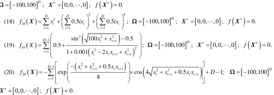
[image:7.595.90.536.87.243.2]

[image:8.595.88.539.99.398.2]

Table 1. The average time contrast of single iteration for the four algorithms (unit: seconds).

fi

MQPAPSO QDPSO PSO SFLA

D = 50 D = 100 D = 50 D = 100 D = 50 D = 100 D = 50 D = 100

f1 0.0186 0.0290 0.0011 0.0019 0.0009 0.0016 0.0014 0.0020

f2 0.0187 0.0292 0.0012 0.0020 0.0012 0.0016 0.0017 0.0025

f3 0.0248 0.0428 0.0064 0.0127 0.0099 0.0227 0.0068 0.0168

f4 0.0188 0.0296 0.0011 0.0019 0.0009 0.0016 0.0014 0.0024

f5 0.0230 0.0397 0.0049 0.0095 0.0016 0.0025 0.0022 0.0043

f6 0.0235 0.0387 0.0018 0.0031 0.0028 0.0048 0.0019 0.0032

f7 0.0187 0.0291 0.0013 0.0021 0.0016 0.0022 0.0014 0.0024

f8 0.0191 0.0295 0.0015 0.0023 0.0019 0.0028 0.0024 0.0036

f9 0.0234 0.0382 0.0016 0.0024 0.0019 0.0028 0.0017 0.0027

f10 0.0193 0.0301 0.0019 0.0031 0.0028 0.0048 0.0017 0.0028

f11 0.0234 0.0383 0.0016 0.0024 0.0016 0.0025 0.0017 0.0027

f12 0.0262 0.0441 0.0096 0.0173 0.0054 0.0089 0.0033 0.0070

f13 0.0193 0.0298 0.0020 0.0030 0.0025 0.0041 0.0017 0.0030

f14 0.0233 0.0372 0.0048 0.0089 0.0028 0.0044 0.0024 0.0033

f15 0.0256 0.0449 0.0031 0.0057 0.0051 0.0096 0.0038 0.0060

f16 0.0248 0.0418 0.0065 0.0124 0.0028 0.0048 0.0027 0.0043

f17 0.0378 0.0706 0.0246 0.0486 0.1116 0.2192 0.0292 0.0651

f18 0.0234 0.0382 0.0017 0.0024 0.0019 0.0025 0.0022 0.0028

f19 0.0206 0.0314 0.0028 0.0037 0.0038 0.0054 0.0033 0.0041

f20 0.0212 0.0320 0.0028 0.0039 0.0041 0.0057 0.0043 0.0052

Table 2. The average optimization results contrast for four algorithms (D = 50).

fi

MQPAPSO QDPSO PSO SFLA

G = 100 G = 100 G = 1000 G = 100 G = 1000 G = 100 G = 1000

f1 1.9E−08 1.5E+03 3.4E−05 3.4E+03 6.0E−05 8.5E+02 0.00108

f2 1.3E−04 9.4E+10 33.1953 3.8E+15 1.3E+02 2.8E+02 2.6E+02

f3 3.7E−09 3.9E+04 1.1E+04 6.7E+04 1.6E+04 6.3E+03 2.5E+03

f4 0.00101 36.9364 10.2029 61.9675 54.6625 12.1258 9.71406

f5 73.2154 1.2E+08 1.3E+02 2.7E+08 2.0E+02 1.1E+07 4.8E+02

f6 4.1E−11 7.2E+07 2.1E+02 3.7E+08 1.5E+05 1.2E+04 2.3E−09

f7 7.9E−06 1.9E+03 2.9E+02 3.3E+03 3.7E+02 1.4E+03 1.0E+03

f8 3.3E−05 21.1629 20.5964 21.2778 21.1744 17.0524 15.7169

f9 4.9E−10 11.1857 0.00352 23.6757 0.03275 2.00564 0.01209

f10 18.5824 2.7E+04 10.5743 6.5E+04 23.4260 1.8E+03 12.7798

f11 2.8E+04 1.6E+06 8.4E+04 5.1E+06 4.2E+05 9.7E+05 2.4E+04

f12 0.18150 2.9E+07 0.28276 6.5E+07 1.65872 1.1E+04 17.3770

f13 7.6E−07 4.2E+03 0.00231 1.0E+04 4.00830 3.2E+03 13.9008

f14 3.9E−11 2.9E+06 7.3E+04 3.9E+07 4.5E+07 8.1E+05 3.4E+04

f15 0.25413 2.3E+02 26.5175 3.0E+02 1.7E+02 1.7E+02 1.5E+02

f16 2.2E−06 1.9E+03 3.5E+02 3.5E+03 3.9E+02 1.3E+03 1.0E+03

f17 0.51201 67.3310 47.5805 78.8131 75.8892 48.0274 33.5393

f18 1.1E−05 8.0E+04 4.1E+04 1.2E+05 9.8E+04 8.0E+03 5.4E+03

f19 1.5E−04 0.49997 0.49959 0.49999 0.49998 0.49469 0.49168

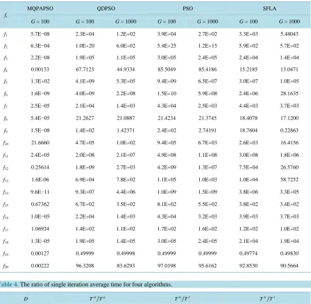
[image:8.595.95.539.420.720.2]

[image:9.595.91.540.99.537.2]

Table 3. The average optimization results contrast for four algorithms (D = 100).

fi

MQPAPSO QDPSO PSO SFLA

G = 100 G = 100 G = 1000 G = 100 G = 1000 G = 100 G = 1000

f1 5.7E−08 2.3E+04 1.2E+02 3.9E+04 2.7E+02 3.3E+03 5.48043

f2 6.3E−04 1.0E+20 6.0E+02 5.4E+25 1.2E+15 5.9E+02 5.7E+02

f3 2.2E−08 1.9E+05 1.1E+05 3.0E+05 2.4E+05 2.4E+04 1.4E+04

f4 0.00133 67.7123 44.9334 85.5049 85.4186 15.2185 13.0471

f5 1.3E+02 4.1E+09 5.3E+05 9.4E+09 6.5E+07 3.0E+07 1.0E+05

f6 1.6E−09 4.0E+09 2.2E+08 1.5E+10 5.9E+08 2.4E+06 28.1635

f7 2.5E−05 2.1E+04 1.4E+03 4.3E+04 2.5E+03 4.4E+03 3.7E+03

f8 5.4E−05 21.2627 21.0887 21.4234 21.3745 18.4078 17.1200

f9 1.5E−08 1.4E+02 1.42371 2.4E+02 2.74191 18.7604 0.22863

f10 21.6660 4.7E+05 1.0E+02 9.4E+05 6.7E+03 2.6E+03 16.4156

f11 2.4E+05 2.0E+08 2.1E+07 4.9E+08 1.1E+08 3.0E+08 1.8E+06

f12 0.25614 1.8E+09 2.7E+03 4.2E+09 1.3E+07 7.5E+04 26.5760

f13 1.6E-06 6.9E+04 7.8E+02 1.1E+05 1.0E+03 1.0E+04 58.7252

f14 9.6E−11 9.3E+07 4.4E+06 1.0E+09 1.5E+09 3.8E+06 3.3E+05

f15 0.67362 6.7E+02 3.5E+02 8.1E+02 5.5E+02 3.8E+02 3.4E+02

f16 1.0E−05 2.2E+04 1.4E+03 4.3E+04 3.2E+03 3.9E+03 3.7E+03

f17 1.06924 1.4E+02 1.1E+02 1.7E+02 1.6E+02 1.2E+02 1.0E+02

f18 1.3E−05 1.9E+05 1.4E+05 3.0E+05 2.4E+05 2.1E+04 1.9E+04

f19 0.00127 0.49999 0.49998 0.49999 0.49999 0.49774 0.49830

f20 0.00222 96.3208 83.6293 97.0198 95.6162 92.8530 90.5664

Table 4. The ratio of single iteration average time for four algorithms.

D M Q

T T M P

T T M S

T T

50 9.863512 9.800094 9.620418

100 9.785713 10.03969 9.752004

AVG 9.824613 9.919894 9.686211

Table 5. The ratio of average optimization results for four algorithms.

D

100

M Q

G

O= O 100

M P

G

O= O 100

M S

G

O= O

2 10

G= 3

10

G= 2

10

G= 3

10

G= 2

10

G= 3

10

G=

50 0.001361 0.165868 0.000671 0.067214 0.002587 0.140945

100 0.000623 0.012133 0.000510 0.000795 0.001124 0.073973

[image:9.595.87.540.624.717.2]

amplitude coding and evolutionary mechanisms can indeed improve the optimization capability. From Table 5, in the same iteration steps, the optimization result of MQPAPSO is only one thousandth of that of QDPSO. On the other hand, in the same running time, the optimization result of MQPAPSO is only nine percent of QDPSO. Experimental results show that multi-bit probability amplitude coding method can indeed significantly improve the optimization ability of the traditional PSO algorithm and other similar algorithms.

8. Conclusion

In this paper, a quantum-inspired particle swarm optimization algorithm is presented encoded by probability amplitudes of multi-qubits. Function extreme optimization results show that under the same running time, the optimization ability of proposed algorithm has greatly superior to the traditional methods, revealing that the multi-qubits probability amplitude encoding method indeed greatly enhances the ability of traditional particle swarm optimization performance.

Funding

This work was supported by the Youth Foundation of Northeast Petroleum University (Grant No. 2013NQ119) and the National Natural Science Foundation of China (Grant No. 61170132).

References

[1] Kennedy, J. and Eberhart, R.C. (1995) Particle Swarms Optimization. ProceedingsofIEEEInternationalConference onNeuralNetworks, New York, November/December 1995, 1942-1948. http://dx.doi.org/10.1109/icnn.1995.488968

[2] Guo, W.Z., Chen, G.L. and Peng, S.J. (2011) Hybrid Particle Swarm Optimization Algorithm for VLSI Circuit Parti-tioning. JournalofSoftware, 22, 833-842. http://dx.doi.org/10.3724/SP.J.1001.2011.03980

[3] Qin, H., Wan, Y.F., Zhang, W.Y. and Song, Y.S. (2012) Aberration Correction of Single Aspheric Lens with Particle Swarm Algorithm. ChineseJournalofComputationalPhysics, 29, 426-432.

[4] Cai, X.J., Cui, Z.H. and Zeng, J.C. (2008) Dispersed Particle Swarm Optimization. Information ProcessingLetters,

105, 231-235. http://dx.doi.org/10.1016/j.ipl.2007.09.001

[5] Liu, Y., Qin, Z. and Shi, Z.W. (2007) Center Particle Swarm Optimization. Neurocomputing, 70, 672-679.

http://dx.doi.org/10.1016/j.neucom.2006.10.002

[6] Zhang, Y.J. and Shao, S.F. (2011) Cloud Mutation Particle Swarm Optimization Algorithm Based on Cloud Model.

PatternRecognitionandArtificialIntelligence, 24, 90-96.

[7] Fang, W., Sun, J., Xie, Z.P. and Xu, W.B. (2010) Convergence Analysis of Quantum-Behaved Particle Swarm Opti-mization Algorithm and Study on Its Control Parameter. ActaPhysicaSinica, 59, 3686-3694.

[8] Sun, J., Wu, X.J., Fang, W., Lai, C.H. and Xu, W.B. (2012) Conver Genceanalysis and Improvements of Quantum- Behaved Particle Swarm Optimization. InformationSciences, 193, 81-103. http://dx.doi.org/10.1016/j.ins.2012.01.005

[9] Lu, T.C. and Yu, G.R. (2013) An Adaptive Population Multi-Objective Quantum Inspired Evolutionary Algorithm for Multi-Objective 0/1 Knapsack Problems. InformationSciences, 243, 39-56. http://dx.doi.org/10.1016/j.ins.2013.04.018

[10] Abdesslem, L. (2013) A Hybrid Quantum Inspired Harmony Search Algorithm for 0-1 Optimization Problems. Journal ofComputationalandAppliedMathematics, 253, 14-25. http://dx.doi.org/10.1016/j.cam.2013.04.004

[11] Gao, J.Q. (2011) A Hybrid Quantum Inspired Immune Algorithmfor Multi Objective Optimization. Applied Mathe-maticsandComputation, 217, 4754-4770. http://dx.doi.org/10.1016/j.amc.2010.11.030

[12] Han, K.H. and Kim, J.H. (2002) Quantum-Inspired Evolutionary Algorithm for a Class of Combinatorial Optimization.

IEEETransactionsonEvolutionaryComputation, 6, 580-593. http://dx.doi.org/10.1109/TEVC.2002.804320

[13] Liu, X.D., Li, P.C. and Yang, S.Y. (2014) Design and Implementation of Quantum-Inspired Differential Evolution Al-gorithm. JournalofSignalProcessing, 30, 623-633.

[14] Eberhart, R.C. and Shi, Y. (2000) Comparing Inertia Weights and Constriction Factors in Particle Swarm Optimization.

ProceedingsofIEEECongressonEvolutionaryComputation, New York, 84-88.

[15] Li, P.C., Wang, H.Y. and Song, K.P. (2012) Research on Improvement of Quantum Potential Well-Based Particle Swarm Optimization Algorithm. ActaPhysicaSinica, 61, Article ID: 060302.