Modelling and Estimation of Spatiotemporal Surface Dynamics Applied to a Middle Himalayan Region

Modelling and Estimation of Spatiotemporal Surface

Dynamics applied to a Middle Himalayan Region

Prashant Kumar

Organisation (CSIO), Sector-30C, Chandigarh-160030,

CSIR, India

Amol P. Bhondekar

Sector-30C, Chandigarh-160030, CSIR, India

Pawan Kapur

Sector-30C, Chandigarh-160030, CSIR, India

ABSTRACT

Accurate and timely estimation of the spatiotemporal surface dynamics is very important for natural resource planning and disaster mitigation. This paper discusses a novel technique to assess the patterns of the surfaces of a particular severe landslide susceptible zone (Kullu-Larji-Rampur geological window, near Aut village, district Mandi, Himachal Pradesh, India; N 31°44’34.78’’ E 77°12’29.02’’). The spatiotemporal surface dynamics of this region, spanning over last 20 years (1989 - 2009), has been modelled using Landsat TM images acquired during summers of 1989, 2000 and 2009. The proposed technique uses image processing to derive regression models of selected area segments, these models are then used to measure area under the curve to estimate the surface area changes. The surface area changes thus obtained have also been validated by standard method of pixel counting. Principal component analysis has been done in order to understand the correlations amongst the estimated parameters, namely; segment lengths, percentage area change and the area change in the first (1989-2000) and second (2000-2009) decades. The results obtained show a fair degree of accuracy as compared to the standard method of pixel counting.

General Terms

Image Processing, Mathematical Modelling, Remote Sensing

Keywords

Digital Change detection, Himalayas, Landsat, Landslides, Remote sensing, Spatiotemporal

1.

INTRODUCTION

Modelling of surfaces can help in assessment and mitigation of Disastrous events. Modelling of surfaces of mountainous regions is a bit complex because of the involvement of several factors such as slope, aspect, relative relief, geological character, drainage, vegetation and land use/land cover [1].

Himalayan mountains being tectonically active are highly prone to landslide activities [1]. Landslide is the most common natural hazard in the region of the study and damages and losses have regularly incurred[2, 3]. The Kullu-Larji-Rampur geological window (KLRW) is severely vulnerable to landslides wherein the rocks are not only highly deformed but the area also possesses active faults [1]. Therefore, a severe landslide susceptible zone falling inside KLRW near Aut village, district Mandi, Himachal Pradesh, India; has been chosen for the current study.

Digital change detection is one of the popular processes in remote sensing applications aimed at identifying spatiotemporal surface dynamics [4, 5]. Wherein, images acquired on the same geographical area at different time intervals are used for the analysis. Change detection approaches are broadly characterized by data transformation procedure and analysis techniques to delineate the area of significant variability. A variety of digital change detection algorithms have been developed so far viz. monotemporal change delineation, delta classification, multidimensional temporal feature analysis, composite analysis, image differencing, image ratioing, multitemporal linear data transformation, change vector analysis, image regression, multitemporal biomass index and background subtraction [5-7]. Digital change detection has been successfully applied to land use change analysis[8-10], natural resource mapping [2, 11] and disaster and damage assessment[12-14].

This work presents a novel technique for area change estimation based upon monotemporal image regression, wherein standard image pre-processing techniques viz. intensity normalization, registration and edge detection are applied to create temporal skeletal images. The skeletal segments of each temporal skeletal image are then segmented and regressed to obtain polynomial models of various orders. The multitemporal polynomial curves for each segment are then superimposed on each other and the area enclosed among them is calculated using integrals. The proposed methodology has been addressed as Integral Method (IM) henceforth. In the present study, the segmentation has been done manually which may be automated and invites research interests for optimum segment selection parameters. The results thus obtained by IM are comparable with the results of standard Pixel Counting Method (PCM).

2.

METHODOLOGY

International Journal of Computer Applications (0975 – 8887) Volume 54– No.7, September 2012

Fig. 1: Major steps of the methodology

2.1

Study Area

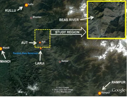
In the present study, a particular severe landslide susceptible zone (KLRW, near Aut village, district Mandi, Himachal Pradesh, India; N 31°44’34.78’’ E 77°12’29.02’’, see Fig. 2) has been considered. Aut is a village in the eastern mountain ranges of Mandi, located on the bank of river Beas, near the confluence of Kullu and Tirthan valleys. The terrain of Aut is steep and hilly. Geologically, it is located in seismic Zone No. IV near a fault line and is prone to earthquakes [15]. The main Kullu Valley is a gently folded antiform having River Beas following its axial plane along a fault running NNW-SSE from the upper catchment to near Aut where it is intersected by a cross fault almost at right angles [16]. This fault is a dextral tear fault with a dislocation of nearly 1.5 km [17]. The rivers Beas, Parbati, Hurla Nala, Sainj Khad, Tirthan Khad etc. follow these fault traces which are well reflected in the trellis like drainage pattern. The area west of river Beas from Bhuntar and south of Parbati River to Rampur along the course of Satluj River is structurally very unique forming window in a window structure [1]. Apart from possessing active faults, the KLRW contains highly deformed rocks and therefore is susceptible to severe landslides [1]. These unique

geological characteristics of the region motivated us to choose the region near Aut for the present study (see inset of Fig. 2).

Fig. 2: Map of Aut (source-Google earth and Google map)

2.2

Preprocessing

2.2.1

Input Image

Input image is a grayscale satellite image. Landsat TM image data files consist of seven spectral bands. The resolution is 30 meters for Bands 1-5, and Band 7. Band 6 resolution (thermal infrared) is a collected 120 meters, but is resampled to 30 meters. When imagery is acquired over large geographic areas, scene differences can and do exist due to different acquisition dates, view angles, sun angles, and atmospheric conditions. Because of this reality, we believe that this form of satellite data is best suited for the analysis of relatively small geographic areas. The appropriate selection of imagery acquisition dates is as crucial to the change detection method as

is the choice of the sensor(s), change categories, and change detection algorithms [6]. Therefore, three cloud-free images corresponding to Landsat path 147, row 38 of the concerned region of the summer season have been taken for each of the years 1989, 2000 and 2009 from U.S. Geological Survey [18]. The images are shown in Fig. 3(a/b/c).

2.2.2

Cropping the area of interest

Fig. 3: Landsat images of Aut, Himanchal Pradesh for the years (a) 1989, (b) 2000 and (c) 2009 and Corresponding cropped images of the actual study site for the years (d) 1989, (e) 2000 and (f) 2009.

2.2.3

Intensity Normalization

In the intensity normalization function that is used to produce the results shown in this paper, the transformation is scaled such that the least intense value in the original image is mapped to a zero intensity value in the normalized image, and, the most intense value in the original image is mapped to an intensity value that is equal to the maximum intensity value determined by the bit depth of the image. This produces results that have a dynamic range that is similar to the one produced by the histogram equalization algorithm [19].

2.2.4

Image Registration

Of all the various aspects of preprocessing for change detection, multidate image registration is one of the most important requirements. The process of image registration is composed of three steps: 1) Sufficient number of control points are prepared; 2) Control points are used to estimate a mapping function between the image to be registered to the reference datum, to a map, or to a reference image; 3) Using the mapping function images are resampled to align with the reference system [20]. Four control points (CPs) have been taken evenly distributed across the entire image for the registration process and the transformation used is affine to maintain the parallelism. The CPs selected included river-intersections, some structure corners, and field boundaries. Control points have been chosen in consultation with a geologist. Accurate registration of multidate imagery is a critical prerequisite of accurate change detection. However, residual misregistration at the below-pixel level somewhat degrades areal assessment of change events at the change/no-change boundaries [6]. The images of the years 2000 and 2009 are registered with the image of year 1989 taking it as a reference image.

2.

2.5

Skeleton formation and Change detection

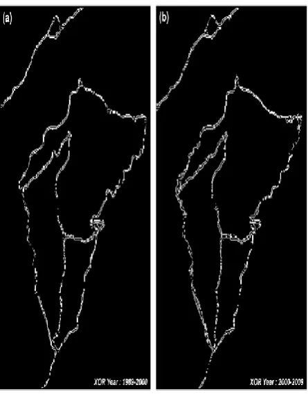
After registration, each image is processed to obtain skeletal edges using Canny’s edge operator [21] for its robustness against noise and efficacy to detect true weak edges. Fig. 4 shows the typical skeletal images of the study region. In order to identify the prospective altered skeletal segments in the first (1989-2000) decade, the skeletal image of the year 1989 has been XORed with the image of the year 2000 (Fig. 5(a)). Similarly, the skeletal image of the year 2000 has been XORed with the image of the year 2009 in order to identify the prospective altered skeletal segments in the second (2000-2009) decade (Fig. 5(b)). These two XORed images have also been further used for area calculation using PCM.

2.3

Segment Selection, Modelling and Area

Estimation

The choice of the segments is a trade-off between their lengths and contour complexities. The smoother the contour, the larger is the segment length and vice versa. Further, choosing too many segments for the sake of accuracy is not advisable and the choice of optimum segments becomes difficult. Therefore the segments are chosen manually. The segment branches in the XORed images having significantly visible changes are identified first and regressed upon (using pixel indices) to derive polynomial equations for each of the branches in the original skeletal images.

International Journal of Computer Applications (0975 – 8887) Volume 54– No.7, September 2012

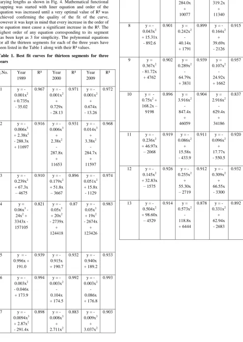
particular order. This process yielded thirteen segments of varying lengths as shown in Fig. 4. Mathematical functional mapping was started with liner equation and order of the equation was increased until a very optimal value of R² was achieved confirming the quality of the fit of the curve, however it was kept in mind that every increase in the order of the equation must cause a significant increase in the R². The highest order of any equation corresponding to its segment has been kept as 3 for simplicity. The polynomial equations for all the thirteen segments for each of the three years have been listed in the Table 1 along with their R² values.

Table 1. Best fit curves for thirteen segments for three years

Seg.No. Year 1989

R² Year 2000

R² Year 2009

R²

1 y =

-0.001x2 + 0.735x

- 35.02

0.967 y = -0.001x2

+ 0.729x - 28.13

0.971 y = -0.001x2

+ 0.674x - 13.26

0.972

2 y =

-0.006x3 + 2.38x2 - 288.3x + 11697

0.916 y = -0.006x3 + 2.38x2 - 287.8x + 11653

0.931 y = -0.014x3 + 3.38x2 - 284.7x + 11597 0.968

3 y =

-0.239x2 + 67.3x

– 4675

0.910 y = -0.179x2 + 51.8x – 3667

0.896 y = -0.051x2 + 15.8x

- 1129

0.974

4 y =

0.06x3 - 24x2 + 3343x - 157105

0.821 y = -0.05x3 + 20x2 - 2739x

+ 124418

0.87 y = -0.05x3 + 19x2 - 2674x

+ 123426

0.983

5 y = -0.996x +

191.0

0.939 y = -0.915x + 190.7

0.932 y = -0.940x + 189.2

0.933

6 y =

-0.003x2 - 0.046x

+ 173.9

0.994 y = -0.003x2

- 0.104x + 174.5

0.992 y = -0.003x2

- 0.086x + 176.8

0.993

7 y =

-0.0094x3 + 2.87x2 - 291.4x

0.898 y = -0.008x3

+ 2.711x2

0.883 y = -0.009x3

+ 3.037x2

0.903

+ 10290 -

284.0x + 10077 - 319.2x + 11340

8 y =

-0.043x2 + 15.31x

- 892.6

0.901 y = 0.242x2

- 40.14x + 1791

0.899 y = -0.164x2

+ 39.69x - 2126

0.915

9 y =

0.367x2 - 81.72x

+ 4762

0.902 y = 0.289x2

- 64.79x + 3831

0.939 y = 0.107x2

- 24.92x + 1662

0.957

10 y = -0.75x2 + 168.2x – 9198

0.896 y = 3.916x2

- 847.4x

+ 46059

0.904 y = 2.916x2 - 629.4x + 34186 0.837

11 y =

-0.236x2 + 46.97x

– 2068

0.919 y = -0.086x2

+ 15.58x - 433.9

0.911 y = -0.096x2

+ 17.77x - 550.5

0.920

12 y =

-0.145x2 + 32.83x

– 1575

0.926 y = -0.255x2

+ 55.30x – 2719

0.912 y = -0.309x2

+ 66.55x - 3300

0.932

13 y =

-0.504x2 + 98.60x

– 4529

0.914 y = 0.573x2

- 118.8x + 6444

0.878 y = -0.331x2

+ 62.94x - 2683

Fig. 5: Change detected by XOR Operation of (a) Im1 (1989) and Im2 (2000) & (b) Im2 (2000) and Im3 (2009)

Fig. 4: Skeletal image of the study region along with identified segments

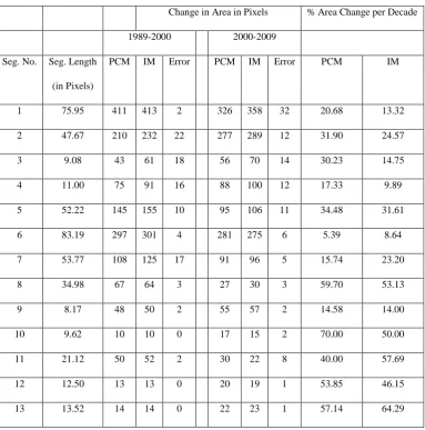
For area change estimation during the two decades, the modelled polynomial equations for each segment are superimposed on each other and the differential area enclosed amongst these curves are calculated using definite integrals as demonstrated in Fig. 6. In order to compare the results obtained by the proposed IM, the change in areas of all the

segments have also been calculated by PCM [23] in the resulting image obtained after the XOR operation (see Fig. 5(a), 5(b)). Both methods show quite similar results. Table 2 shows the results obtained by PCM and IM; and their comparisons in terms of absolute error and the percentage change in the area for each of the thirteen segments

International Journal of Computer Applications (0975 – 8887) Volume 54– No.7, September 2012

Table 2. Comparison of Area Change estimated by PCM and IM

Change in Area in Pixels % Area Change per Decade

1989-2000 2000-2009

Seg. No. Seg. Length

(in Pixels)

PCM IM Error PCM IM Error PCM IM

1 75.95 411 413 2 326 358 32 20.68 13.32

2 47.67 210 232 22 277 289 12 31.90 24.57

3 9.08 43 61 18 56 70 14 30.23 14.75

4 11.00 75 91 16 88 100 12 17.33 9.89

5 52.22 145 155 10 95 106 11 34.48 31.61

6 83.19 297 301 4 281 275 6 5.39 8.64

7 53.77 108 125 17 91 96 5 15.74 23.20

8 34.98 67 64 3 27 30 3 59.70 53.13

9 8.17 48 50 2 55 57 2 14.58 14.00

10 9.62 10 10 0 17 15 2 70.00 50.00

11 21.12 50 52 2 30 22 8 40.00 57.69

12 12.50 13 13 0 20 19 1 53.85 46.15

13 13.52 14 14 0 22 23 1 57.14 64.29

3.

RESULTS AND DISCUSSION

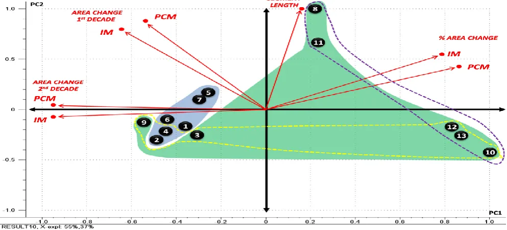
In order to understand the correlation among the various parameters such as segment lengths, percentage area change and the area change in the first decade (1989-2000) and the second decade (2000-2009), principal component analysis has been done. PCA is a statistical technique helpful in understanding multivariate data. It captures the relevant information in a set of input data providing a lower dimension, but informative representation of the original data. It sequentially creates a set of principal components from the original data. The first principal component (PC1) maps the maximum variance and information of the input data followed by the other principal components (PC2, PC3 and so on) in descending order of the variance [24]. Generally a good explanation of the data is mapped by the first two principal components, i.e. PC1 and PC2. In order to understand, the relationships between the samples and variables, a PCA bi-plot is generally used. In the bi-bi-plot, the loadings for each variable can be presented as vectors, superimposed upon the scores plot for the same PCs. The length of the loading vector of a variable signifies its importance; the angles between the vectors show the relationships between the variables themselves, and the vector direction is indicative of the correlations between variables and samples. Close and extreme placements of the loading vectors of the variables, suggest a positive and negative correlation respectively

amongst them. Similarly, the loading vectors which are perpendicular to each other through the origin are independent. Loadings close to the PC axis are significant only to that PC and variables with a large loading on both the PCs are significant to them. Statistical software The Unscrambler 9.7 has been used here for the PCA.

respectively in both the decades. In general, the blue and the green segments also show a low and a high percentage area change respectively in the second decade, segments 9 and 3 being exceptions. This confirms the fact that any smaller change in a bigger segment is not reflected significantly whereas the same smaller change in a smaller segment is reflected significantly in the form of percentage change. This also explains the placement of segment lengths loading vector in the first quadrant along with percentage area change vectors. The segments (i.e. 8, 10, 11, 12 and 13) with relatively higher percentage change per decade have been marked by dotted violate boundary. Amongst these segments, the segments 8 and 11 are relatively larger segments in comparison to segments 10, 12 and 13. The reason for a larger percentage change for segments 10, 12 and 13 is that they are smaller segments, so any smaller change in them will be reflected as a larger change. Also, segments 8 and 11 are steeper sections causing a relatively larger change [25]. Further, the segments whose area change has increased in the second decade (i.e. 2, 3, 4, 9, 10, 12 and 13) have been marked by yellow dotted boundary and the segments outside

this boundary have shown a decrease in the area. One of the possible reasons for decrease in area can be the reduction in vegetation. The other region is the type of soil presence in those segments which has been examined during the field inspection and it was found that there were clay soils in the segments where surface area changes have reduced. As far as increase in the surface area is concerned; one of the possible reasons can be the accumulation of soils fallen from very elevated and steeper sections of the mountain to less elevated sections [25, 26]. The segments 8, 10, 11, 12 and 13 become the major susceptible zones for landslide occurrences because a higher percentage shift in the area shows that there are very less vegetation in these segments [27, 28], also confirmed by scouting data. Shifting has been quite random for different segments and it involves many natural and man-made factors (viz. snowfall, cloud burst, urbanisation, intense rainfall, vegetation change, earthquake, erosion of lateral margins) for its random behaviour which can be modelled provided there is sufficient data corresponding to each factor. Further research is needed to model the contribution of all the factors that actually cause shifting in the area.

Fig. 7: PCA bi-plot plotted using parameters of Table 2

4.

CONCLUSIONS

A novel technique for area change estimation has been applied to a severe landslide susceptible zone. This technique can be used for its capability to measure the spatial and temporal changes in a mountainous region and to subsequently determine an effective means to measure landscape stability. Landslide susceptibility maps can be produced based on stability of the segments. The technique has been compared with the standard method of pixel counting and satisfactory results have been obtained. The accuracy of the proposed technique may further be improved by optimum selection of segments. However, optimum selection of the segments still remains a major challenge and needs further research.

5.

ACKNOWLEDGEMENTS

We gratefully acknowledge the support extended by CSIR-Central Scientific Instruments Organization, Chandigarh.

6. REFERENCES

[1] V. B. S. Chandel, K. K. Brar, and Y. Chauhan, “RS & GIS Based Landslide Hazard Zonation of Mountainous Terrains A Study from Middle Himalayan Kullu District, Himanchal Pradesh, India,” International Journal of Geomatics and Geosciences, vol. 2, no. 1, 2011.

[2] R. R. Bharti, B. S. Adhikari, and G. S. Rawat, “Assessing vegetation changes in timberline ecotone of Nanda Devi National Park, Uttarakhand,” International Journal of Applied Earth Observation and Geoinformation, no. 0, 2011.

International Journal of Computer Applications (0975 – 8887) Volume 54– No.7, September 2012

[4] R. S. Lunetta, J. F. Knight, J. Ediriwickrema et al., “Land-cover change detection using multi-temporal MODIS NDVI data,” Remote Sensing of Environment, vol. 105, no. 2, pp. 142-154, 2006.

[5] A. Singh, “Review Article Digital change detection techniques using remotely-sensed data,” International Journal of Remote Sensing, vol. 10, no. 6, pp. 989-1003, 1989/06/01, 1989.

[6] P. R. Coppin, and M. E. Bauer, “Digital change detection in forest ecosystems with remote sensing imagery,” Remote Sensing Reviews, vol. 13, no. 3-4, pp. 207-234, 1996/04/01, 1996.

[7] T. R. Martha, N. Kerle, V. Jetten et al., “Characterising spectral, spatial and morphometric properties of landslides for semi-automatic detection using object-oriented methods,” Geomorphology, vol. 116, no. 1–2, pp. 24-36, 2010.

[8] B. Ahmed, and R. Ahmed, “Modeling Urban Land Cover Growth Dynamics Using Multi‑Temporal Satellite Images: A Case Study of Dhaka, Bangladesh,” ISPRS International Journal of Geo-Information, vol. 1, no. 1, pp. 3-31, 2012.

[9] M. E. Bauer, B. C. Loffelholz, and B. Wilson, Estimating and Mapping Impervious Surface Area by Regression Analysis of Landsat Imagery, p.^pp. 488: CRC Press, 2007.

[10] P. Griffiths, P. Hostert, O. Gruebner et al., “Mapping megacity growth with multi-sensor data,” Remote Sensing of Environment, vol. 114, no. 2, pp. 426-439, 2010.

[11] M.-K. Kim, and J. Daigle, “Detecting vegetation cover change on the summit of Cadillac Mountain using multi-temporal remote sensing datasets: 1979, 2001, and 2007,” Environmental Monitoring and Assessment, vol. 180, no. 1, pp. 63-75, 2011.

[12] F. Fiorucci, M. Cardinali, R. Carlà et al., “Seasonal landslide mapping and estimation of landslide mobilization rates using aerial and satellite images,” Geomorphology, vol. 129, no. 1–2, pp. 59-70, 2011. [13] S. Ghosh, C. J. van Westen, E. J. M. Carranza et al.,

“Generating event-based landslide maps in a data-scarce Himalayan environment for estimating temporal and magnitude probabilities,” Engineering Geology, vol. 128, no. 0, pp. 49-62, 2012.

[14] C. J. van Westen, E. Castellanos, and S. L. Kuriakose, “Spatial data for landslide susceptibility, hazard, and vulnerability assessment: An overview,” Engineering Geology, vol. 102, no. 3–4, pp. 112-131, 2008.

[15] A. Emerson, G. C. L. Howell, and H. L. Wright, Gazetteer of the Mandi State, New Delhi: Indus Publishing, 1998.

[16] M. Sah, and R. Mazari, “An overview of the geoenvironmental status of the Kullu Valley, Himachal

Pradesh, India,” Journal of Mountain Science, vol. 4, no. 1, pp. 003-023, 2007.

[17] R. Shankar, and K. J. S. Dua, “On the Existence of a Tear Fault Along Upper Beas Valley, District Kulu, Himachal Pradesh, and its Bearing on the Thermal Activity,” Himalayan Geology, vol. 8, no. 1, pp. 466-472, 1978.

[18] United States Geological Survey. http://www.usgs.gov/.

[19] R. C. Gonzalez, R. E. Woods, and S. L. Eddins, Digital Image Processing Using MATLAB, p.^pp. 827: Gatesmark Publishing, 2009

[20] T. Kim, and Y.-J. Im, “Automatic satellite image registration by combination of matching and random sample consensus,” IEEE Transactions on Geoscience and Remote Sensing, vol. 41, no. 5, pp. 1111- 1117 2003. [21] J. Canny, “A Computational Approach to Edge Detection,” Pattern Analysis and Machine Intelligence, IEEE Transactions on, vol. PAMI-8, no. 6, pp. 679-698, 1986.

[22] A. Carrara, M. Cardinali, R. Detti et al., “GIS techniques and statistical models in evaluating landslide hazard,” Earth Surface Processes and Landforms, vol. 16, no. 5, pp. 427-445, 1991.

[23] N. Sarkar, and B. B. Chaudhuri, “An efficient differential box-counting approach to compute fractal dimension of image,” Systems, Man and Cybernetics, IEEE Transactions on, vol. 24, no. 1, pp. 115-120, 1994. [24] A. P. Bhondekar, M. Dhiman, A. Sharma et al., “A novel

iTongue for Indian black tea discrimination,” Sensors and Actuators B: Chemical, vol. 148, no. 2, pp. 601-609, 2010.

[25] R. Soeters, and C. J. van Westen, "LANDSLIDES: INVESTIGATION AND MITIGATION," SLOPE INSTABILITY RECOGNITION, ANALYSIS, AND ZONATION, A. K. Turner and L. R. Schuste, eds., pp. 129-177: Transportation Research Board, 1996.

[26] F. C. Dai, and C. F. Lee, “Landslide characteristics and slope instability modeling using GIS, Lantau Island, Hong Kong,” Geomorphology, vol. 42, no. 3–4, pp. 213-228, 2002.

[27] J. B. Adams, D. E. Sabol, V. Kapos et al., “Classification of multispectral images based on fractions of endmembers: Application to land-cover change in the Brazilian Amazon,” Remote Sensing of Environment, vol. 52, no. 2, pp. 137-154, 1995.