Volume 51– No.19, August 2012
A Study on the Effect of Regularization Matrices in
Motion Estimation
Alessandra Martins Coelho
Instituto Federal de Educacao, Ciencia e Tecnologia do Sudeste de Minas Gerais (IF Sudeste MG), Av. Dr. José Sebastião da Paixão,s/n°, Lindo Vale CEP: 36180-000, Rio Pomba, MG, Brazil
Vania V. Estrela
Universidade Federal Fluminense (UFF), Praia Vermelha, Niteroi, RJ, CEP 24210-240, Brazil
ABSTRACT
Inverse problems are very frequent in computer vision and machine learning applications. Since noteworthy hints can be obtained from motion data, it is important to seek more robust models. The advantages of using a more general regularization matrix such as =diag{1,…,K} to robustify
motion estimation instead of a single parameter λ (=I) are investigated and formally stated in this paper, for the optical flow problem. Intuitively, this regularization scheme makes sense, but it is not common to encounter high-quality explanations from the engineering point of view. The study is further confirmed by experimental results and compared to the nonregularized Wiener filter approach.
General Terms
Pattern Recognition, Image Processing, Inverse Problems, Computer Vision, Error Concealment, Motion Detection, Machine Learning, Regularization.
Keywords
Regularization, inverse problems, motion estimation, image analysis, computer vision, optical flow, machine learning.
1.
INTRODUCTION
Motion provides significant cues to understand and analyze scenes in applications such as sensor networks, surveillance [18], image reconstruction, deblurring/restoration of sequences [6, 9], computer-assisted tomography, classification [16], video compression and coding [9]. It may help characterize the interaction among objects, collision course, occlusion, object docking, obstructions due to sensor movement, and motion clutter (multiple moving objects superfluous to the investigation).
A block motion approach (BMA) [9] relies on dividing an image in blocks and assigning a motion vector (MV) to each of them, but BMAs often separate visually meaningful features. Dense optical flow or pel-recursive schemes comprise another important family of motion analysis methods [1, 2, 14]. An optical flow (OF) method assigns a unique MV to each pixel to overcome some of the limitations of BMAs. Intermediary frames can be constructed afterwards by resampling the image at places determined by linear interpolation of the motion vectors existent between adjacent frames. pel-recursive approaches allows for management of motion vectors with sub-pixel accuracy.
Consider the motion model
zGu
with Gm×n (m≥n). The least-squares (LS) estimate uLS is obtained from the known observed data vector zm by minimizing the functional
JLS(u)=║z-Gu║2
2
. If, for a full rank overdetermined system,
uLS=(G
TG)-1GTz = G†z (1)
exists, where G†=(GTG)-1GT is the pseudo-inverse of G, then
uLS might be a poor approximation due to several sources of error. Very often, G is ill-conditioned or singular and z is the result of noisy measurements [3, 5, 14, 15] caused by nonlinearities in the system and/or modeling deficiencies. The effect of the conditioning of G can be better understood if one looks at its SV decomposition (SVD) of G as follows:
G=UPVT, (2) where the m×n matrix P has entries Pii=pi, with pi≥0 for i
= 1, 2, …, min(m, n) and other entries are zero. The pi’s are
the SVs of G (which are equal to the eigenvalues of GT G). U
m×m
has m orthogonal eigenvectors of GGT
as its columns. V
n×n
has n orthogonal eigenvectors of GT
G as its columns. Then, uLS can be written as (for further explanations, see [7, 17, 18]):
with (UTz)
i being the i-th entry of vector UTz and Vi standing
for the i-th column of matrix V. If G is ill-conditioned, then at least one of its SVs will be very small when compared to the others. Now, when z is an outlier with errors in its i-th component, the corresponding term (UTz)i will be magnified
even more if the i-th singular value (SV) is very small. The calculation of (GTG)-1 can be a difficult task due to this noise amplification phenomenon. Although this text deals with the theoretical aspects of regularization, it should be pointed out that in our specific problem (motion estimation), where Gis a gradient matrix. The entries of G are spatial derivatives of the image intensity and it is a well-known fact that differentiation is a noise-inducing operation. Hence, the matrix inversion required by the LS solution [7] presents two sources of error: the ill-posedness of the problem and the use of a matrix whose entries are obtained through differentiation.
Regularization allows solving ill-posed problems because it transforms them into well-posed ones, that is, problems with unique solutions [5, 10, 13] and guaranteed stability when numerical methods are called for. Given a system z=Gu+b, regularization tries to solve it by introducing a regularization
uLS =VP
-1 UTy=
i p 0 i
1 p
Volume 51– No.19, August 2012 term relying on a priori knowledge about the set of admissible
solutions [7, 11] in order to compensate the ill-posed nature of a matrix G while constraining the admissible set of solutions [1]. There is a relationship between regularization parameters and the covariances of the variables involved. The advantages of the use of a more general regularization matrix
=diag{1,…,K} instead of a single parameter λ (=I) for
the OF problem are investigated and formally stated. In the next section, the underlying model for the optical flow estimation problem is stated. Section 3 presents a brief review of previous work done in regularization of estimates, where the simplest and most common estimators are analyzed: the ordinary least squares (OLS), besides one of its enhanced versions, the regularized least squares (RLS), here referred to as uOLS and uRLS, respectively [5, 9, 10-12, 14]. Section 4 shows
some experiments attesting the performance improvement of the proposed algorithm. To conclude, a discussion of the results is considered in Section 5.
2.
MOTION ESTIMATION
The displacements of all pixels between adjacent video frames form the displacement vector field (DVF). OF estimation can be done using at least two successive frames. This work aims at determining the 2D motion resultant from the noticeable motion of the image gray level intensities.
Pel-recursive algorithms are predictor-corrector-type of estimators [2, 7, 14] which function in a recursive manner, pursuing the direction of image scanning, on a pixel-by-pixel basis. Initial estimates for a given point can be projected from other neighboring pixels motions. It is also possible to devise additional prediction schemes that correct an estimate in agreement with some error measure resultant from the displaced frame difference (DFD) and/or other criteria. It was stated before that a picture element belongs to a region undergoing movement if its brightness has changed between successive frames k-1 and k. The motion estimation strategy is to discover the equivalent brightness value Ik(r) of the k-th
frame at position r = [x, y]T, and consequently, the exact displacement vector (DV) at the working point r in the current frame which is given by d(r) = [dx, dy]T. Pel-recursive
algorithms seek the minimum value of the DFD function contained by a small image part together with the working point and presume a constant image intensity along the motion path. The DFD correspond to the gradient defined by (r;d(r))=Ik(r)-Ik-1(r-d(r))
and the ideal registration of frames will give the subsequent answer: Ik(r)=Ik-1(r-d(r)). The DFD characterizes the error
attributable to the nonlinear temporal estimate of the brightness field through the DV. It should be mentioned that the neighborhood structure (also called mask) has an effect on the initial displacement estimate.
The relationship linking the DVF to the gray level field is nonlinear. An estimate of d(r), is achieved straightforwardly with minimization of r,d(r)) or via the determination of a linear relationship involving these variables through some model. This is consummated using a Taylor series expansion of Ik-1(r-d(r)) with reference to the position (r-di(r)), where di(r) stands for a guess of d(r) in i-th step which yields (r; r
-di(r)) -uT Ik-1(r- di(r)), or in its place
(r; r-di(r)) = -uT I
k-1(r- di(r))+e(r, d(r)), (4)
where the displacement update vector is given by u=[ux, uy]
T
= d(r) – di(r). e(r,d(r)) corresponds to the error from pruning
the higher order terms (linearization error) of the Taylor =[δ/δx, δ/δy]T stands for the spatial
gradient operator at r. The update of the motion estimate is founded on the DFD minimization at some pixel. Without supplementary suppositions on the pixel motion, this estimation problem comes to be ill-posed as a result of the succeeding problems: a) model nonlinearities; b) the answer to the 2D motion estimation problem is not unique due to the aperture problem; and c) the solution does not continuously rely on the data due to the fact that motion estimation is extremely sensitive to the presence of observation noise in video images.
Applying Equation (4) to all points in the surrounding the current pixel and taking into account an error term n∈m
yields
z=Gu+n, (5) where the gradients with respect to time r, r-di(r)) have
been piled to compound the z∈Nincluding DFD particulars inside an N-pixel neighborhood , the N×2 G results from stacking the gradients with respect to spatial coordinates at each observation, and the error term amounts to the N×1 noise vector n which is considered Gaussian with n~N(0, σn2IN).
Each row of G has entries [axi, ayi]
T
, with i = 1, …, N. A bilinear interpolation scheme [2, 14] provides the spatial gradients of Ik-1. The assumptions made about n for LS
estimation are: zero expected value (E(n) = 0), and Var(n) =
E(nnT) = σ2IN. IN is an N×N identity matrix, and n
T is the transpose of n.The earlier expression emphasizes the fact the observations are erroneous or noisy and it will be of help once introducing the concept of regularization and expanding it. Each row of G has entries fk-1(r) corresponding to a given
pixel location within a mask. The components of the spatial gradients are computed through a bilinear interpolation scheme [2, 14]. The preceding expression will permit introducing the concept of regularization and extending it.
3.
ANALYSIS OF THE ESTIMATORS
Previous works [3-6, 10] have shown that regularization improves LS estimates for ill-posed problems because they reduce the sensitivity of uRLS to perturbations in z, the
instability and the non-uniqueness of inverse problems by introducing prior information via the regularization operator
Q and the regularization parameter λ>0. For the linear model from Equation (5), uRLS results from the minimization of
Jλ(u)= ║z-Gu║2
2+λ║
Qu║2
2
, whose solution is given by
uRLS (λ)= (G T
G+λQTQ)-1GTz. (6) The essential idea behind this method is recognizing a nonzero residual |z-Gu|, provided the functional Jλ(u) is
minimum. The regularization factor λ directs the weight given to the minimization of the smoothness term ||Qu||2
2
compared with the minimization of the residual ||z-Gu||2. The simplest form of regularization is to assume ΛRLS=λQTQ=λI. The solution uRLS(λ) is no longer unbiased, and it can introduce
useful prior knowledge about the problem, which is captured by the additional qualitative operator Q. In most cases, Q is chosen with the intention that the new solution is smoother than the one obtainable by the ordinary LS (OLS) approach. This function is likely to encompass a few regularity properties as by way of illustration: continuity and differentiability. λ→0 leads to uLS and λ→∞ implies that
Volume 51– No.19, August 2012 The regularization parameter turns out to resurface as a
variance quotient, and this permits estimation via variance component estimation techniques as discussed in [3, 11]. The consequential formulas are similar to those frequently seen in deconvolution of sequences. A modern treatment from a practical standpoint can be seen, e.g., in [17, 18].
3.1
Error Analysis of the RLS Estimate
For the specified observation model, the LMMSE solution from [3, 7] is equivalent to Equation (6):
uLMMSE = RuG
T
(GRuG
T
+Rn)
-1
z. (7)
uLS requires knowledge of the covariance matrices of the parameter term (Ru) and the noise/linearization error term
(Rn), respectively. The most common assumptions when
dealing with such problem is to consider that both vectors are zero mean valued, their components are uncorrelated among each other, with Ru = σu2I and Rn= σn2I where σu2 and σn2
are the variances of the components of the two vectors. Using the matrix inversion lemma [7], one can show that the RLS and the LMMSE solutions are identical if λQTQ=Rn (Ru)
-1
as stated in [3, 7, 10, 11]. The Linear Minimum Mean Squared Error (LMMSE) for the linear observation model is also the maximum a posteriori (MAP) estimate, when a Gaussian prior on u is assumed and the noise n is also Gaussian (for more details, see [3, 11]). If u=0, Ru= diag(σu1
2
, σu2 2
), and
Rn= σ 2
I, then Equation (7) becomes
uRLS(Λ)= (G T
G+Λ)-1GTz, (8) with Λ = diag(σ2/σ
u1 2,σ2/σ
u2 2)=λI.
3.2
Analysis of the RLS Estimate with
Diagonal Λ
The mean square error of uRLS is E{L1
2
}=E{(uRLS -u) T
(uRLS-u)}.
Applying the unitary transformation
T = Mu, (9)
with M=VT, where V comes from the singular value decomposition from Equation (2), such that
GTG=MTP2M=VP2VT, then we can define
G=G*M, and (10) z=G*t+n. (11) This transformation reduces the system to a canonical form and simplifies some analyses due to the diagonalization of some matrices. It follows from Equation (10) that
G*TG*=(GM-1)TGM-1=M-TGTGM-1
= M-TMTP2MM-1=P2, and (12) = tTt=(Mu)TMu=uTMTMu=uTu. (13)
The expression for E{L1
2
} can be more easily developed if one keeps in mind the fact that it is invariant under orthogonal transformations like its shown in Equation (9): E{L1
2
}= E{(uRLS-u) T
(uRLS-u)}= E{(tRLS-t)
T
(tRLS-t). (14) The RLS estimate of t, for the model in Equation (11) is given by
tRLS= RtG*T[G*RtG*T+ Rn]-1z. (15)
Equations (10) to (15) result in μt=μu=0 and Rt=E{ttT}=E{MuuTMT}=MRuMT. Obviously, Equation
(15) can be restated as follows:
tRLS = [Rt
-1
+G*T σ -2G*]-1G*T σ -2z, (16) = [t+G*TG*]-1G*Tz (17) =M[+GTG]-1GTz (18) The last equation confirms the obvious result
tRLS = MuRLS, (19)
where no longer conforms to the definition provided in Section 3.1. The transition between Equations (16) and (18) takes into consideration Equation (12) and the relationship below
t= σ
2
Rt
-1 = σ 2
M-TRu
-1
M-1=MMT . (20) Furthermore, if we assume that
tLS=[ G
*T
G*]-1G*Tz, (21)
Z*=[I+(G*TG*)-1Λ
t]-1=I- ΛtW*, and (22)
W*=[G*TG*+Λt]-1, then we have (23)
tRLS = Z
*
tLS . (24) Combining Equations (14) and (10) yields
E{L1
2
}= E{( Z*tLS-t)
T
(Z*tLS-t)}. (25) = E{tLST Z
*T
Z*tLS +t
T
t - 2 tLST Z
*T
-t}
= σ2Tr{(G*TG*)-1Z*TZ*}+tT(Z*-I)T(Z*-I)t. (26)
With the help of Equations (12), (22) and (23), it is possible to write
E{L12}=σ2Tr{P-2[I+(G*TG*)-1Λt]-T[I+(G*TG*)-1Λt]-1}
+tT W*TΛ
tTΛt W*t. (27)
The use of a canonical form makes the above calculations easier because all matrices are diagonal and leads to
E{L1 2}=σ2
Tr{P-2[I+P-2Λt] -2
} +tT Λt 2
[P2+Λt]
-2
t. (28) E{L12}= E{L1*2} can be enunciated in terms of the SVs of G,
that is, pi’s, the nonzero entries λti of the regularization matrix
Λt of the transformed system and the individual components
of the transformed unknown tas follows:
2 2 2
2 2
1 2 2 2 2
1 1
{ }
( ) ( )
i
i i
n n
i t i
i i t i i t
t p
E L
p p
. (29)Alternatively,
E{L1*2(Λt)}= γ1(Λt) + γ2(Λt) , (30)
where
2 2
1 2 2
1
( )
( i)
n i i i t
p p
t , and (31)
2 2
2 2 2
1
( )
( )
i i n
i t i i t
t p
t
. (32)
The earlier decomposition will be helpful in analyzing the properties of uRLS and tRLS in the succeeding theorems.
THEOREM 1. The total variance γ1(Λt) is the sum of the
variances of all the entries of tRLS, that is, γ1(Λt) is the sum of
all the elements of the main diagonal of matrix Rt RLS [5, 11].
PROOF: The covariance matrix of tRLS can be obtained from
Volume 51– No.19, August 2012
Rt RLS=σ
2
Z*[G*TG*]-1Z*T. (33) Each diagonal entry of Rt RLS contains the variance of the i-th
component of tRLS, that is, tRLS(i) and their sum is
2 1
1
{ ( )} { } { [( ) ] ( ) }
n
* * T * * T i
Var i Tr Tr
tRLS R$tRLS Z G G Z$ .
Combining the previous expression with Equations (2), (12), (22) and (23) yields
2 * * 1 * * * *
1
{ ( )} {[ ] { } [ ] }
n
T T T T T
i
Var i Tr
$tRLS G G t G G G G t
2
2 2 2
2 2
1
{ [ ] }
( i)
n i i i t
p Tr p
2 2 tP P ,
(34)
which agrees with Equation (31). Thus, γ1(Λt) is the sum of
variances of all the entries of tRLS and it is also the sum of all
elements along the diagonal of Equation (33).
COROLLARY 1. The total variance is the same in the
original basis and in the canonical system, that is
γ1(Λt) = γ1(Λ) . (35)
PROOF: Equations (11), (28), (26), and (30) result in
2 1 2 1 { ( )} { } { } { } ( ). n T u i
Var u i Tr Tr
Tr
RLS RLSRLS
RLS t
t t
R MR M
R $ $ $ $ Defining
Z=((GTG)-1Λ+I)-1, then Equations (1), (11), and (35) imply that uRLS =Z uLS =Z(G
T
G)-1GTz. We can rewrite E{L12} in terms of uRLS as
E{L1
2
}= E{(uRLS -u) T
(uRLS -u)}
= σ2Tr{(GTG)-1ZT Z}+uT(Z-I)T(Z-I)u
= σ2Tr{(GTG+ Λ)-1}- σ2Tr{(GTG+ Λ)-1Λ(GTG+ Λ)-1} + ║Λ(GTG+ Λ)-1u║2
2 . (37)
Similarly to what was done before E{L1
2
}= E{( uRLS -u) T
(uRLS -u)}=γ1(Λ)+ γ2(Λ),
where γ1(Λ)= σ2Tr{(GTG)-1ZT Z} (38)
= σ2Tr{(GTG+ Λ)-1}- σ2Tr{(GTG+ Λ)-1Λ(GTG+ Λ)-1},
and
γ2(Λ)= ║Λ(GTG+ Λ)-1u║2
2
. (39)
RuRLScan be written likewise to Equation (33):
RuRLS= σ 2
Z(GTG)-1ZT. (40) Additionally,
2 1 2 1
{ u } { ( T ) T} {( T ) T }
Tr Tr Tr
RLS
R$ Z G G Z G G Z Z ,
where it was used the property that for two k×k matrices C
and D we have Tr{CD}=Tr{DC}. Comparing Equations (32), (38), (41) and using some of the results from Theorem 3 yield γ1(Λt)= γ1(Λ). Thus, γ1(Λ) is the sum of variances of all the
entries of uRLS which is the sum of all elements along the
main diagonal of RuRLS.
COROLLARY 2. The total variance is independent of the
basis chosen.
PROOF: It follows promptly from Corollary 3.
THEOREM 2. As Λ tends to 0, that is, the regularization tends to none, the value of E{L12} approaches the sum of the
diagonal entries of the covariance matrix for the LS estimate of u. In mathematical terms [3, 5, 11]:
2 2
1 2
1
1 lim { } { }
n
i i
E L Tr
p
uLS
Λ 0 R$ . (41)
PROOF: When Λ approaches 0, the last two terms of
Equation (36) become zero and what is left is 2 2 1
1
lim { } {( T ) }
E L Tr
Λ 0 G G . (42)
The covariance matrix of the LS estimate of uis given by RuLS= E{ uLSuLS
T
}E{(GTG)-1GTzzTG(GTG)-1} = σ2
(GTG). (43) Comparing the previous two equations results in
2 1
lim { }E L Tr{ }
$uLS
0
R . Since GTG=VP2VT we also have
2 1 1 2 2 2 1 ( ) { } {( ) } 1 { } n T i n i i
ii Tr Tr
Tr p
LS LS u u 2R R G G
P
$ $
verifying thus the theorem.
COROLLARY 3. As Λt tends to 0, the sum of the diagonal
entries of the covariance matrix for the LS estimate of t is equal tothe sum of the diagonal entries of the covariance matrix for the LS estimate of u:
2
2
1 1 1
1
( ) ( )
n n n
i i i i
ii ii
p
Ru$LS
R$tLS
. (45)PROOF: First let us notice that RtLS =M RuLSM
T
, so that
1
( ) { } { }
n
i
i Tr Tr
R$tLS R$tLS Ru$LS (46)2 1 2 2
2 1 1 {( ) } { } n T i i Tr Tr p
2
A A P ,
(47)
which agrees with Equation (45). (36)
Volume 51– No.19, August 2012
THEOREM 3. The total variance γ1(Λt) is a continuous,
monotonically decreasing function of the entries of the main diagonal of Λt, that is, λti, i=1,…,n [5].
PROOF: The first derivative of γ1(Λt) with respect to λti can
be obtained from Equation (31) and it equals to
2 2 1
2 3
2
( )
i i
p p
ti ti
.
COROLLARY 4. The first derivative with respect to λti of
the total variance γ1(Λt) approaches -∞ as λti0, and pi20.
PROOF: In the neighborhood of the origin this derivative is
negative and it is given by
2 1
4 0
lim 2
i
p
ti i
t
, and 2 1
0 , 0
lim
i p
ti ti
.
THEOREM 4. The squared bias γ2(Λt) is a continuous,
monotonically increasing function of λti, i=,…,n [5, 11].
PROOF: The squared bias γ2(Λt) is defined in Equation (32).
The denominator of γ2(Λt) is always positive because pi
2
>0 for all values of i and λti≥0, provided GTG is orthogonal (no
singularities in the denominator). The function exists at the origin: γ2(0)=0. γ2(Λt) can be rewritten as
2
2 2
2 1
( )
1
n
i i
i
t p
i
t
t
Λ . (50)
The terms pi2/λti are monotone decreasing for increasing λti’s. Hence, γ2(Λt) is monotone increasing.
COROLLARY 5. The first derivative with respect to λti of
the squared bias γ2(Λt) is zero at the origin as λti0+.
PROOF: The first derivative of γ2(Λt) with respect to λti can
be obtained from Equation (32) and it equals to
2 4 2 3
2
2 3
( 2 )
2
( )
i i i
i
t p p
p
i i i i
i i
t t t t
t t
.
Around the origin this derivative is zero:
2
0
lim 0
ti i
t
.
COROLLARY 6. The squared bias γ2(Λt) approaches uTu as
an upper limit when the solution is oversmoothed, that is, Λt
→diag{∞,…,∞}.
PROOF: Rewriting γ2(Λt) as in Equation (50), the pursued
limit becomes
2 2
( ,..., )
1
lim ( )
n
T T T T
i diag
i
t
t
t
Λ Λ t t u M Mu u u.
COROLLARY 7. ║RtRLS║2 is smaller than║RtLS║2 for Λt>0.
PROOF: According to linear algebra, ║G║2=λGMAX, where
λGMAX is the largest SV of G. From Equations (10) and (43), it
follows that
║RtLS║2 =σ2Tr{P -2}.
If pn is the smallest SV of G, then
║RtLS║2 =σ
2
/pn2. (51)
Similarly, by looking at Equation (33) we obtain ║RtRLS║2 = σ2pn2 /(pn2+ λtn)
2.
The analysis of the two previous expressions shows that the introduction of the regularization factor λtn damps the
denominator of ║RtRLS║2 when compared to ║RtLS║2 .
COROLLARY 8. The use of a regularization matrix Λt
reduces the variances of the entries of uRLS when compared to
the variances of the entries of uLS.
PROOF: Comparing Equations (36) and (46) shows that
Var{ uRLS(i)}, i = ,…,n is damped by the corresponding λtiof
Λt. As a result, Var{uRLS(i)}, is smaller than Var{uLS(i)}.
Therefore, the RLS estimate has smaller error than the LS estimate.
THEOREM 5. There always exists a matrix Λt= diag{λt1, …,
λti, …, λtn} where λti >0 and a constant k > 0, such that
2 2 2 2 2
1 1 1
1
{ ( )} { ( )} { ( )} {1 }
n i
[image:5.595.61.270.77.434.2]E L Λt E L kI E L 0
p .Volume 51– No.19, August 2012
PROOF: Two cases need investigation: Λt =kI and Λt
=diag{λt1, …, λti, …, λtn}. First, let us evaluate
2 2 2 2 2 2 2 2 2
1
1 1
{ ( )} { ( ) } / ( )
n n
i i i i
E L kI
p p k k
t p k . From the previous expression, we have
2 2 2
1
1
{ ( )} {1 }
n i
E L 0
p . (52) First, let us analyze the case λt1= … = λti= … = λtn = k. Thenecessary and sufficient condition to have E{L1
2
(kI)}< E{L1
2
(0)} is that there always exists a k>0 such that dE{L1
2
(kI)}/dk<0:
2 2 2 2
2 1
2 3 2 3
1 1
{ ( )}
2 2 0
( ) ( )
n n
i i i
i i
dE L k p t p
k
dk
p k
p k I
. (53)
Since σ2 is a constant, dE{L
1
2(kI)}/dk will receive more
contribution of the term involving the entry ti with the largest
absolute value tmax=|ti|max. Therefore,
2 2 2
2 2 2
max
2 3 2 3
1
( )
( )
2 2 0
( ) ( )
n
j i i
i j
p kt p kt
p k p k
which results in ktmax2- σ2<0 or similarly k<σ2/ tmax2. By
inspection, it is easy to verify that γ1(Λt) is monotonically
decreasing with Λt , which means that γ1(0) is always greater
than γ1(Λt) provided ti >0, i = 1,…,n. For γ2(Λt), one can
observe that the term (P2+Λt)
-1
when viewed as a matrix whose entries are polynomials, will have terms with denominators greater or (in the worst case) equal to their numerator. The result of adding γ1(Λt) and γ2(Λt) will be
always smaller than γ1(0) +γ2(0)=σ
2
{ / }
n 2 i i 1
1 p
. Now, let us look at the case t=diag{t1,…,ti,…,tn}. Similarly to whatwas done for the case t1=…=ti=…=tn=k, we have that
2 2 2 2
2 1
2 3 2 3
1 1
{ ( )}
2 2 0
( ) ( )
n n
i i i
i i
dE L p t p
d
p i
p i i i
t
t
t t t
Λ
.
By inspecting Equation (51), we conclude that dE{L1
2
(Λt)}/dλti
< 0 when λti= σ 2
/ti
2
. If at least one ti is such that ti >k= σ2
/tmax2, then inspection of Equation (53) leads to
E{L1
2(Λ t)}<E{L1
2(kI)}.The previous theorems and corollaries
show that E{L1
2
(Λt)} has a minimum.
4.
EXPERIMENTS
In this section, we present several experimental results that illustrate the effectiveness of the proposed approach and compare it to the Wiener filter (LS) estimate [7, 13] and the case ΛRLS=λI. The algorithms were tested on a synthetic QCIF
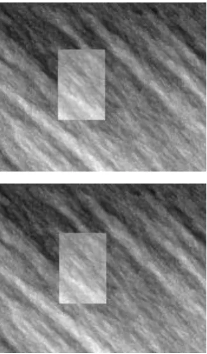
sequence (144×176, 8-bit). Two consecutive frames of this synthetic sequence are shown in Figure 1. In this sequence, there is a moving object in a moving background. It was created using the following auto-regressive model:
f(m,n) = 0.333[f(m,n-1) + f(m-1,n) + f(m-1,n-1)] + n(m,n). For the background, n is a Gaussian random variable with mean 1 = 50 and variance 12 = 49. The rectangle was
generated with 2 = 100 and variance 22= 25.
Fig 2: Motion error obtained for the Wiener filter top),
ΛRLS=λI (middle) and Λ=diag {λ1,…, λi, …, λN} (bottom)
for the noiseless version of the "Synthetic" sequence.
It has been shown (that Ordinary Cross Validation (OCV) in some cases does not provide good estimates of consult [2, 4, 8] for more details). A modified method called Generalized Cross Validation (GCV) function gives more satisfactory results (see, for example, [2, 3, 4, 8]) and it is given by
2
2 2
( ) 1
( ) 1
{ ( )} GCV
N Tr N
I A
I A
,
where A(Λ)= G[GTG+Λ]GT.
Volume 51– No.19, August 2012 (MSE) and bias in the horizontal and vertical directions can
evaluated. These metrics are given by
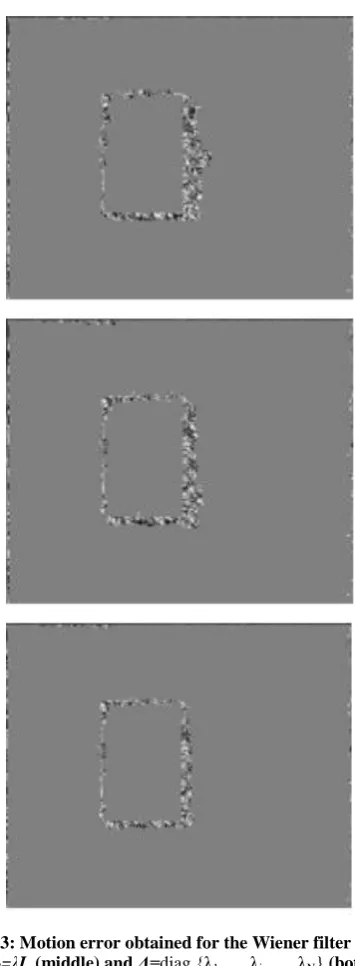
Fig 3: Motion error obtained for the Wiener filter top),
ΛRLS=λI (middle) and Λ=diag {λ1,…, λi, …, λN} (bottom)
for the "Synthetic" sequence with SNR =20dB.
2
1
[ ( ) i( )]
i i
MSE d d
MN
r S
r $ r , and
1
[ ( ) i( )]
i i
bias d d
MN
r S
r $ r ,
where S is the entire frame and i=x,y. The average mean-squared DFD defined as
2 1
2 2
[ ( ) ( ( ))]
(# )(# )
K
k k
k AVG
f f
DFD
ofPixels ofFrames
rkr r d r
,
and the average improvement in motion compensation (IMCAVG) in dB given by
2 1 2
10
2 1
2
[ ( ) ( )] 10log
[ ( ) ( ( ))]
K
k k
k
AVG K
k k
k
f f
IMC
f f
k
k
r
r
r r
r r d r
[image:7.595.76.254.107.591.2].
Table 1. Results for different implementations, SNR = ∞
(noiseless).
Wiener λI Λdiagonal
MSEx 0.1548 0.1534 0.1493
MSEy 0.0740 0.0751 0.0754
biasx 0.0610 0.0619 0.0581
biasy -0.0294 -0.0291 -0.0294
IMCAVG 19.46 19.62 19.89
[image:7.595.339.520.362.485.2]DFDAVG2 4.16 4.05 3.76
Table 2. Results for different implementations, SNR
=20dB.
Wiener λI Λdiagonal
MSEx 0.2563 0.2544 0.2437
MSEy 0.1273 0.1270 0.1257
biasx 0.0908 0.0889 0.0881
biasy -0.0560 -0.0565 -0.0561
IMCAVG 14.74 14.83 15.15
DFDAVG2 12.24 12.02 11.16
Figure 2 shows the error frames estimated by subtracting the true frame 2 from predicted ones. The resulting motion vector estimates were obtained via the Wiener filter (LS), ΛRLS=λI
and Λ=diag {λ1,…, λi, …, λN} without noise. Table 1
illustrates the values for the MSE’s, biases, IMCAVG (dB) and
DFDAVG2 for the estimated optical flow in this case. Likewise,
Figure 3 and Table 2 present results when SNR = 20dB.
5.
CONCLUSIONS
In general, finding a numerical solution for an ill-posed problem involves regularization. A better-conditioned one subsequently approximates the original problem. Some distances or divergences metrics are often used as measures of closeness between problems. In this paper, the consequences of regularization upon the quality of the RLS estimators have been analyzed in order to bridge the gap between the simplest form of regularization λQTQ=λIN=ΛRLS - where λ>0 is a scalar
regularization parameter and Q is a regularization operator – and a solution Λ=λQTQ=diag {λ1,…, λi, …, λN} in terms of
the analysis of the goodness of the solution. Equation (20) relates a diagonal Λ to Λt via a unitary transformation. It is
important to point out that our analysis is valid for the case when Λt belongs to the subspace of matrices that can be
[image:7.595.104.232.630.684.2]Volume 51– No.19, August 2012 This work applies the proposed regularization method using a
matrix Λ to the optical flow estimation problem. Indeed, experiments showed that the MSE, and biases were smaller for
Λ=diag {λ1,…, λi, …, λN}. The quality of the estimates of the
motion vectors can be seen from the values of IMCAVG and
DFDAVG2.
The bias-variance tradeoff must be taken into consideration for RLS estimates. Nevertheless, the proposed linear model brings in biases from two sources: the risk/penalty function (the Euclidean norm amplifies errors due to outliers, especially when near a decision limit), and regularization. A way of decreasing biases is to increase variance, but it may introduce overfitting. It was confirmed by experiments that the expected value of the errors and biases were lowered when a regularization matrix Λ was used.
The analysis done so far did not evaluate the effects of preconditioning and scaling on the RLS estimate. The application of variational methods such as total variation minimization is more difficult, given that it is not easy to determine straightforward and useful preconditioners for the problem.
A video sequence may have various non-informative and spurious features that can obliterate the understanding of its main features. The model studied, can benefit from techniques such as cross validation to find the optimal hyperparameters. Depending on the problem nature and model assumptions, small singular values can be discarded in order to reduce the dimensionality of the system to be solved. This procedure is called Truncated SVD (TSVD) [12, 17, 18].
6.
ACKNOWLEDGEMENTS
The authors thank FAPERJ and CAPES for their support.
REFERENCES
[1] Biemond, J., Looijenga, L., Boekee, D.E., and Plompen, R. H. J. M. 1987. A pel-recursive Wiener-based displacement estimation algorithm, Signal Processing, 13, 399-412.
[2] Estrela, V. V., Rivera, L.A., Beggio, P.C., and Lopes, R.T. 2003. Regularized pel-recursive motion estimation using generalized cross-validation and spatial adaptation, In Proc. of SIBGRAPI 2003 XVI Brazilian Symp. Comp. Grap. and Image Processing, 331-338.
[3] Galatsanos, N.P., and Katsaggelos, A.K. 1992. Methods for choosing the regularization parameter and estimating the noise variance in image restoration and their relation, IEEE Trans. Image Proc., Vol. 1, No. 3, 322-336.
[4] Golub, G.H., Heath, M. and Wahba, G. 1979. Generalized cross-validation as a method for choosing a good ridge parameter, Technometrics, Vol. 21, No. 2, 215-223.
[5] Hoerl, E., and Kennard, R.W. 1970. Ridge regression: biased estimation for nonorthogonal problems, Technometrics, 55-67.
[6] Katsaggelos, A.K. 1991. Image Restoration, Springer-Verlag, Berlin-Heidelberg, Germany.
[7] Kay, S. 1993. Fundamentals of Statistical Signal Processing: Estimation Theory, Prentice Hall.
[8] Reeves, S.J. 1992. A cross-validation framework for solving image restoration problems, J. Vis. Comm. Im. Repres., Vol. 3, No. 4, 433-445.
[9] Tekalp, M. 1995. Digital Video Processing, Prentice Hall.
[10]Tikhonov, A., and Arsenin, V. 1977. Solution of Ill-Posed Problems, John Wiley and Sons, 1977.
[11]Thompson, A.M., Brown, J.C., Kay, J.W., and Titterington, D.M. 1991. A study of methods for choosing the smoothing parameter in image restoration by regularization, IEEE Trans. P.A.M.I., Vol. 13, No. 4, 326-339.
[12]Van Loan, C.F., and Golub, G. H. 1993. Matrix Computations, The John Hopkins University Press. [13]Wiener, N. 1948. Cybernetics, MIT Press, Cambridge,
MA.
[14]Coelho, A. M. and Estrela, V. V. 2012. Data-driven motion estimation with spatial adaptation, International Journal of Image Processing (IJIP), vol. 6, no. 1. http://www.cscjournals.org/csc/manuscript/Journals/IJIP/ volume6/Issue1/IJIP-513.pdf
[15]Bharathi P.T. and Subashini, P. 2012. Automatic identification of noise in ice images using statistical features, Proc. SPIE 8334, 83340G http://dx.doi.org/10.1117/12.946038
[16]Padmavathi, V., Subashini, P. and Krishnaveni, M. 2011. A generic framework for landmine detection using statistical classifier based on IR images, International Journal on Computer Science and Engineering (IJCSE), Vol. 3 No. 1, 254-261, ISSN : 0975-3397 http://www.enggjournals.com/ijcse/doc/IJCSE11-03-01-164.pdf
[17]Franz, M. O., and Schölkopf, B. 2006. A unifying view of Wiener and Volterra theory and polynomial kernel regression. Neural Computation 18(12): 3097-3118. http://keck.ucsf.edu/~craig/Franz_Scholkopf_2006_A_U nifying_View_of_Wiener_and_Volterra_Theory_and_Po lynomial_Kernel_Regression.pdf