Chance Constrained Linear Plus Linear Fractional Bi level Programming Problem

Chance Constrained Linear Plus Linear Fractional

Bi-level Programming Problem

Surapati Pramanik

Department of Mathematics, Nandalal Ghosh B.T. College,

Panpur, P.O.- Narayanpur, District – North 24 Parganas,

Pin Code-743126, West Bengal, India

Durga Banerjee

Ranaghat Yusuf

Institution,Rathtala,P.O.-Ranaghat,District-Nadia,Pin Code-741201,West Bengal,

India

Bibhas C. Giri

Department of Mathematics, Jadavpur University, Kolkata –

700032, West Bengal, India

ABSTRACT

We present fuzzy goal programming approach to solve chance constrained linear plus linear fractional bi-level programming problem. The chance constraints with right hand parameters as random variables of prescribed probability distribution functions are transformed into equivalent deterministic system constraints. We construct nonlinear membership functions based on deterministic system constraints. The nonlinear membership functions are transformed into linear membership functions by using first order Taylor’s series approximation. In the bi-level decision making context, decision deadlock may arise due to the dissatisfaction of the lower level decision maker with the decision of upper level decision maker. To overcome this problem, decision maker of each level gives his preference bounds on decision variables under his/her control to provide some relaxation on their decisions. Fuzzy goal programming model is used to achieve highest membership goals by minimizing negative deviational variables. Euclidean distance function is used in order to find out the most satisfactory solution. We solve a chance constrained linear plus linear fractional bi-level programming problem to illustrate the proposed approach.

General Terms

Bi-level programming, linear plus linear fractional programming.

Keywords

Bi-level programming, linear plus linear fractional programming, chance constraints, fuzzy goal programming, Taylor’s series.

1.

INTRODUCTION

In game theory, inventory problems, production house problems, banking systems, the objective functions may be either linear fractional or the sum of linear and linear fractional functions. In 1962, Charnes and Cooper [1] developed variable transformation method to solve multi-objective linear fractional programming problem (MOLFPP). Linear programming with a fractional objective function was studied by Bitran and Noveas [2] in 1973. Goal programming (GP) approach to linear fractional criteria was introduced by Kornbluth and Steuer [3]. In GP, the goals are stated explicitly. In real situation, the target goals may not be explicitly stated due to uncertainty. To deal with uncertainty, Luhandjula [4] proposed fuzzy approaches for solving MOLFPP. Sakawa and Kato [5] used interactive decision making to solve MOLFPP involving fuzzy numbers.

In 1970, Teterav [6] first studied optimality criteria for solving linear plus linear fractional programming problem. Schaible [7] studied the sum of linear and linear fractional

function in 1977. Chadha [8] and Hirche [9] developed different models for solving the sum of linear and linear fractional programming problem. Under fuzzy constraints, linear plus linear fractional programming problem (LPLFPP) was studied by Jain and Lachhwani [10]. In 2010, Jain and Lachhwani [11] developed LPLFPP with homogeneous constraints using fuzzy approach. Jain et al. [12] discussed multi-objective linear plus linear fractional programming problem (MOLPLFPP) containing non-differential term. In 2011, Singh et al. studied fuzzy goal programming (FGP) approach for solving MOLPLFPP. Using Taylor’s Series approximation Pramanik et al. [14] developed FGP model to solve MOLPLFPP. Recently, Pramanik and Banerjee [15] studied chance constrained MOLPLFPP based on first order Taylor’s series approximation.

Linear plus linear fractional bi-level programming problem (LPLFBLPP) is a special type of non-linear bi-level programming problem. In this paper, we consider the objective function of each level DM as linear plus linear fractional function. We also consider the constraints as linear functions and probabilistically defined. There are many research fields where LPLFBLPP arises such as robust data fitting, traffic assignment problems, portfolio optimizations, banking systems, any management systems, etc.

In this paper, the concept of Pramanik and Banerjee is extended to chance constrained linear plus linear fractional bi-level programming problem (CCLPLFBLPP). In bi-bi-level programming problem (BLPP), two types of decision makers (DMs) i.e. upper level decision maker (ULDM) and lower level decision maker (LLDM) execute their decision in hierarchical way. Each level DM independently controls a set of decision variables. Candler and Townsley [16] as well as Fortuny –Amart and McCarl [17] developed the formal BLPP. After that many researchers [18, 19] studied BLPP in various perspectives. Sakawa and Nishizaki [20, 21] introduced linear fractional BLPP using interactive fuzzy programming. Pramanik and Dey [22] presented bi-level linear fractional programming problem based on FGP using first order Taylor’s series approximation.

formulated and Euclidean distance function is used to determine the most compromise solution. A numerical example is solved to demonstrate the proposed approach.

The rest of the paper is developed in the following way. In Section 2, we formulate CCLPLFBLPP. In Section 3, chance constraints are reduced into equivalent deterministic constraints. Non-linear membership functions are constructed in Section 4. In Section 5, technique of linearization of non- linear membership function is discussed by using first order Taylor’s series. In Section 6, preference bounds on the decision variables are defined. Section 7 is devoted to develop two FGP models for solving CCLPLFBLPP. The Euclidean distance function is described in the next Section 8. The step wise description of the process for solving CCLPLFBLPP is presented in the Section 9. Section 10 presents illustrative numerical example of CCLPLFBLPP. Section 11 presents conclusion and future work.

2.

FORMULAON OF CCLPLFBLPP

CCLPLFBLPP can be presented as:

[ULDM]MaxZ (X)

1 1 X

=

β x d

α x c ) γ x p (

1 T 1

1 T 1 1 T 1

  

 (1)

[LLDM] MaxZ(X)

2 2

X _β

x d

α x c ) γ x p (

2 T 2

2 T 2 2 T 2

  

 (2)

subject to X∈ X`=

} 0

≥

X , m -I > ) d

≥ ≤

X C P r( : R

∈

X

{ n (3)

Here, p , ₁T p T₂ c , 1T T 2

c T

1

d , T 2

d ∈Rn and

1

α ,

2

α

,

₁

,

₂

,

1



,

2

 are constants. The decision vector X = (x1 11, x12,

x13,…, x1n1) is controlled by ULDM and X = (x₂ 21, x22,

x23,…, x2n2) is controlled by LLDM. X₁∪X₂=X

n R

∈ , n1

+ n2 = n, ‘T’ means transposition of vector. I, d ,mare

vectors of order p



1, every elements of Iis unity. Cis the given matrix of order p n. The polyhedron X’ is assumed to be non-empty and bounded.

3.

REDUCTION OF STOCHASTIC

CONSTRAINTS INTO EQUIVALENT

DETERMINISTIC CONSTRAINTS

We consider the chance constraints of the form:

Pr (

i n

1 j cijxjd



 ) ≥ 1-mi, i = 1, 2, …, p1. (4)

 Pr (

) d var(

) d ( E -d

≤

) d var(

∑c x -E(d)

i i i

i n

1 =

j ij j i

) ≥ 1-m_i, i = 1, 2,…, p1

) ) d var(

) d ( E -d

≤

) d var(

∑_{c x -E(d )}

P r( -1

≥

m

⇒

i i i

i n

1 =

j ij j i i

) ) d var(

) d ( E -d > ) d var(

∑_{c x -E(d)}

P r(

≥

m

⇒

i i i

i n

1 =

j ij j i i

) d var(

∑c x -E(d)

≥

) m ( Ψ

⇒

i n

1 =

j ij j i i

1

-∑_{c x -E(d)} ≥

) d var( ) m ( Ψ

⇒

n

1 =

j ij j i i

i 1

-∑c x ≤_{E(d )+Ψ (m) var(d)}

⇒

n

1 =

j i i

1 -i j

ij ,

i = 1, 2, …, p1 (5)

Here, (.) and Ψ (.) represent the distribution function and -1 inverse of the distribution function of standard normal variable respectively.

We consider the case when

Pr (

i n

1 j ij j

d x c 



 )

≥

1- mi,i = p1 +1, p1 +2, …, p. (6)

The constraints can be rewritten as:

Pr (

) d var(

) d ( E -d

≥

) d var(

∑c x -E(d)

i i i

i n

1 =

j ij j i

)

≥

1- m_i , i = p1+1, p1 +2,

…, p.

i i

n

1 =

j ij j i

m -1

≥

) ) d var(

∑c x -E(d)

( Ψ

⇒

i i

n 1 =

j ij j i

m -1

≥

) ) d var(

∑_{c x -E(d )}

(-Ψ -1

⇒

) d var(

∑c x -E(d)

≥

) m ( Ψ

⇒

i n

1 =

j ij j i i

1

-∑c x ≥E(d)-Ψ _{(m) var(d)}

⇒

n

1 =

j i i

1 -i j

ij , (7)

i = p1 + 1, p1 + 2,…, p.

X≥

0

(8) Let us denote the equivalent deterministic system constraints (5), (7) and (8) by X. Here, X` and X are equivalent set of constraints.

4.

CONSTRUCTION OF MEMBERSHIP

FUNCTIONS

In order to construct non-linear membership function subject to the equivalent deterministic system constraints, the objective functions are maximized separately.

Let the individual best solution for the objective function )

X ( Z

i

,

i = 1, 2 be

2 , 1 = i , ) x ,..., x , x ,..., x , x , x ( =

X B

in B

1 + i in B

i in B

3 i B

2 i B

1 i B

Let maxZ(X)=Z =Z(XB) 1 1 B 1 1 X ∈ X and ). X ( Z = Z = ) X ( Z max B 2 2 B 2 2 X ∈ X

If we consider the individual best solution as the aspiration level, the fuzzy goal assumes the form:

) X ( Z

i



_~ B i Z

,i = 1, 2 (9)

) X ( Z = Z B 1 1 B

1 and Z =Z(X ) B 2 2 B

2 are the upper tolerance limits

of the fuzzy objective goals of ULDM and LLDM respectively. Similarly, W

1

Z = Z(XB)

2 1 and

W 2

Z =Z₂(X₁B) are the lower tolerance limits of the fuzzy objective goals of ULDM and LLDM.

Now, the membership function for the objective function )

X ( Z

1 of ULDM can be written as:

Z ≤ ) X ( Z if , 0 , Z ≤ ) X ( Z ≤ Z if , Z -Z Z -) X ( Z , Z ≥ ) X ( Z if , 1 = ) X ( μ W 1 1 B 1 1 W 1 W 1 B 1 W 1 1 B 1 1

1 (10)

and the membership function for the objective function )

X ( Z

2 of LLDM can be formulated as:

Z ≤ ) X ( Z if , 0 , Z ≤ ) X ( Z ≤ Z if , Z -Z Z -) X ( Z , Z ≥ ) X ( Z if , 1 = ) X ( μ W 2 2 B 2 2 W 2 W 2 B 2 W 2 2 B 2 2

2 (11)

Now, the CCLPLFBLPP reduces to max (X)

1

 ,

maxμ₂(X), subject to

X∈X. (12)

5.

CONVERSION OF NON-LINEAR

MEMBERSHIP FUNCTION INTO

LINEAR MEMBERSHIP FUNCTION BY

USING TAYLOR’S SERIES

APPROXIMATION

LetX = (x ,x ,x ,...,x ,x ,...,x*) ,i=1,2 in * 1 + i in * i in * 3 i * 2 i * 1 i *

i be the

individual best solution of i(X)subject to the equivalent deterministic system constraints. Then we transform the non- linear membership function (X)

i

 into an equivalent linear

membership function *(X)

i

 at the point * i

X by using first order Taylor’s series as follows:

( )

X

μ₁ ≅μ₁ X*1 + μ X x ∂ ∂ ) x -x

( ₁ *1 1 * 11 1 + ) x -x ( * 12

2 ∂_x μ X

∂ *

1 1 2

+…+(x -x* ) 1 1n 1

n

( )

* 1 1 1 n X μ x ∂ ∂ + ) x -x ( * 1 + 1 1n 1 + 1

n

( )

* 1 1 1 + 1 n X μ x ∂ ∂ +...

+(x_n-x_1n* ) ₁

( )

*1 n X μ x ∂ ∂

= μ*(X)

1 (13)

( )

X μ

2 ≅

( )

* 2 2X

μ +(x -x* ) 21

1

( )

* 2 2 1 X μ x ∂ ∂

+(x -x* ) 22 2

( )

* 2 2 2 X μ x ∂ ∂

+…+(x -x* ) 2 2n 2

n ∂_x μ

( )

X +

∂ * 2 2 2 n ) x -x ( * 1 + 2 2n 1 + 2

n

( )

* 2 2 1 + 2 n X μ x ∂ ∂

+…+

(

x

-

x

*

)

2n n

( )

* 2 2 n X μ x ∂ ∂

=μ*₂(X) (14)

6.

PREFERENCE BOUNDS ON THE

DECISION VARIABLES

Since the objectives of level DMs are conflicting, cooperation between the level DMs is necessary in order to reach compromise optimal solution. Each DM tries to reach maximum profit with the consideration of benefit of other. Cooperation between the DMs is reflected by the relaxations provided by the level DMs on both decision variables.

Let (x -r_) j 1 *

j

1 and

(

x

+

r

)

+ j 1 *

j

1 (j = 1, 2, …, n1) be the

lower and upper bounds of decision variable

x

_1j(j = 1, 2, …,

n1) provided by the ULDM.

) x ,..., x , x ,..., x , x ( = X * n 1 * 1 + 1 n 1 * 1 n 1 * 12 * 11 *

1 is the individual best

solution of the non-linear membership functionμ₁(X)of

ULDM when calculated in isolation subject to the equivalent deterministic system constraints.

Similarly, (x -r_) j 2 *

j

2 and

(

x

+

r

)

+ j 2 *

j

2 (j = 1, 2, …, n2)

be the lower and upper bounds of decision variables j 2 x

(j = 1, 2, …, n2) provided by the LLDM. ) x ,..., x , x ,..., x , x ( = X * n 2 * 1 + 2 n 2 * 2 n 2 * 22 * 21 *

2 is the individual best

solution of the non-linear membership functionμ₂(X)of

LLDM when calculated in isolation subject to the equivalent deterministic system constraints. Therefore, preference bounds on the decision variable can presented as follows:

) r -x ( _ j 1 * j

1  x1j



(

x

+

r

+

)

j 1 *

j

1 (j = 1, 2, …, n1) (15)

) r -x

( *_{2j 2}__j 

j 2

x ( x*_2j+r₂+_j )(j = 1, 2, …, n2) (16)

Here, _

j 1

r

, +

j 1

r

(j = 1, 2, …, n1) and

_ j 2 r , +

j 2

r (j = 1, 2, …, n2 )

are all of non-negative values and these are not necessarily same.

7.

FORMULATION OF FGP MODEL OF

CCLPLFBLPP

The CCLPLFBLPP reduces to the following problem: Maxμ*₁(X), Max μ*(X)

2

) r -x ( _

j 1 *

j

1 x1j( x +r )

+ j 1 *

j

1 , (j = 1, 2, …, n1)

)

r

-x

(

_

j 2 *

j

2 x2j

(

x

+

r

)

+

j 2 *

j

2 , (j = 1, 2, …,n2)

X∈_{X (17)}

According to Pramanik and Dey, it can be written [23] as: ,

1 d

i * i 

 

i = 1, 2. (18)

_ 1 d and _

2

d are the negative deviational variables. Now, two

FGP models are formulated as follows: Model-I

min  ₍₁₉₎ subject to

, 1 = d + ) X (

μ _

1 * 1

, 1 = d + ) X (

μ _

2 * 2

λ ≥ _ 1 d ,

λ ≥ _ 2

d

,

, 1

≤

d

≤

0 ₁_

, 1

≤

d

≤

0 ₂_

) r -x

( _

j 1 *

j 1



j 1

x ( x₁*_j+r₁+_j ), (j = 1, 2, …, n1)

)

r

-x

(

_

j 2 *

j

2 x2j

(

x

+

r

)

+

j 2 *

j

2 , (j = 1, 2, …,n2)

X∈X

Model –II (20)

Min

ξ

= 

 

2 1 i i

d

subject to , 1 = d + ) X (

μ _

1 * 1

, 1 = d + ) X (

μ _

2 * 2

, 1

≤

d

≤

0 _ 1

, 1

≤

d

≤

0 ₂_

) r -x

( _

j 1 *

j

1 x1j( x +r )

+ j 1 *

j

1 , j = 1, 2, …, n1

) r -x

( *_{2j 2}__j 

j 2

x 

(

x

+

r

+

)

j 2 *

j

2 , j = 1, 2, …,n2

X∈X

8.

USE OF DISTANCE FUNCTION TO

DETERMINE COMPROMISE

SOLUTION

For multi objective programming, the objectives are incommensurable and conflicting in nature. The aim of decision makers is to find out the compromise solution which is as near as possible to the ideal solution points in the decision making context. Here, we use the Euclidean distance function [24] of the type

D2=

2 / 1 2

1 i

2 * i)

1 ( _

 

 

 (21)

The solution with the minimum distance is considered as the best compromise optimal solution.

9.

SUMMARIZATION OF THE

PROCESS FOR SOLVING CHANCE

CONSTRAINED LPLFBLPP

To solve CCLPLFBLPP we use the following steps.

Step-1. Transform the chance constraints into equivalent deterministic constraints.

Step-2. Calculate individual best solution for each linear plus linear fractional objective function of the level DM subject to the equivalent deterministic constraints.

Step-3. Lower and upper tolerance limits are determined for each linear plus linear fractional objective function as stated in Section 4.

Step-4. Non linear membership functions are formulated by using individual best solutions subject to the equivalent deterministic system constraints.

Step-5. Find out the individual best solution for each of the non-linear membership functions subject to the equivalent deterministic constraints.

Step-6. Using first order Taylor’s series, the non-linear membership functions are approximated into linear functions at the individual best solution point.

Step-7. Both level DMs express their choices for the upper and lower preference bounds on the decision variables controlled by them.

Step-8. Two FGP models are formulated and solved.

Step-9. Determine the Euclidean distance for two optimal compromise solutions obtained from two FGP Models.

Step-10. Select the solution with the minimum Euclidean distance as the best compromise optimal solution.

10.

ILLUSTRATIVE EXAMPLES OF

CCLPLFBLPP

To illustrate the proposed FGP approach, the following CCLPLFBLPP with maximization type objective function at each level is considered.

2 1

2 1 2 1

1

x x +x 3x -2x + x + 8 = ) X ( Z max [ULDM]

(22)

2 1

2 1 1

2 2

x 3x +x

x 2 -x -7 + x = ) X ( Z max ] LLDM

[ (23)

subject to

Pr (4x1 +3x2 ≤ d1) ≥ 1-

1

m

(24)

Pr (5x1 +2x2 ≥ d2 ) ≥ 1- m (25)₂

x1≥0, x2≥0, (26)

The mean, variance and the confidence levels are prescribed as follows:

E (d1) = 2, var (d1) = 1,

1

m = 0.02 (27)

E (d2) = 4, var (d2) = 2,

2

Using (5) and (7), the chance constraints defined in (24) and (25) can be converted into equivalent deterministic constraints as:

4x1 + 3x2 ≤ 4.055 (29)

5x1 +2x2 ≥ 1.518055 (30)

The individual best solution for each objective function of the level DM subject to the equivalent deterministic constraints is obtained as Z₁B=10, at B

1

X = (0.303611, 0), and B

2

Z 9, at

B 2

X = (0, 0.7590275). The fuzzy goals appear as:

) X ( Z

1



_~10, Z2(X)



_~ 9 (31) The lower tolerance limits are obtained as ZW 5.759028

1 

and ZW 6.970278.

2 

Now, the non-linear membership function for ULDM and LLDM are constructed as follows:

= ) X ( μ

1

5.759028 ≤

) X ( Z if 0

, 10 ≤ ) X ( Z ≤ 5.759028 if

, 5.759028

-10

.759028 5 -) X ( Z

, 10 ≥ ) X ( Z if 1,

1

1 1

1

(32)

= ) X ( μ₂

6.970278

≤

) X ( Z if 0

, 9

≤

) X ( Z

≤

6.970278 if

, 6.970278

-9

6.970278

-) X ( Z

, 9

≥

) X ( Z if 1,

2

2 2

2

(33)

The non-linear membership functions μ (X)

1 and μ2(X)are linearized at their individual best solution point at B

1

X =

(0.303611, 0), B 2

X = (0, 0.7590275) and we obtain equivalent linear membership functions as follows:

) X (

* 1

 = 1 + (x1 –0.303611) * 0 + (x2 -0) * (0.303611-5) /

(4.240972*0.33611), (34)

) X (

* 2

 = 1 + (x1-0) * (0.7590275-7) / (2.029722*0.7590275)

+ (x2 –0.7590275) ×0 (35)

Let 0 ≤ x1≤ 0.5 and 0 ≤ x2 ≤ 1 be the preference bounds

provided by the level DMs.

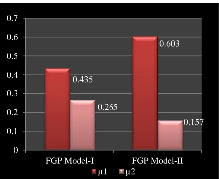
[image:5.595.315.542.109.250.2]

By using two FGP models (19) and (20), the optimal compromise solutions (See Figure –1, Fifure-2 and Figure-3) are presented in the Table1.

Table 1. The optimal solutions obtained from two FGP models of the problem

Model

No. 1

μ ,

2 μ x ,

1 x2 Z1,Z2 D2 FGP-I 0.435

0.265

0.2102191 0.2334797

7.6024 7.5073

0.928

FGP-II 0.603 0.157

0.2468549 0.1418902

8.3169 7.3289

0.932

Comparing Euclidean distance D2 (see Table 1), we conclude

that model I offers better optimal solution than Model II for this problem.

[image:5.595.312.545.288.412.2]

Figure 1. Comparison of optimal solutions

Figure 2. Comparison of optimal solutions

Figure 3. Comparison of obtained resulting membership values

11. CONCLUSION

In this paper, we present CCLPLFBLPP in simple way. The proposed approach is very easy to understand. In the proposed approach, chance constraints are transformed into equivalent deterministic constraints and linear plus linear fractional bi-level programming problem is converted into linear bi-bi-level programming problem by using the first order Taylor’s series approximation.

For the further study, chance constrained multi-level linear plus linear fractional programming problem can be solved by

10

7.6024 8.3169

9

7.5073 _7.3289

0 2 4 6 8 10 12

Maximum value

FGP Model-I FGP Model-II Z1

Z2

10

7.6024 8.3169 9

7.5073 7.3289

0 2 4 6 8 10 12

Maximum value

FGP Model-I

FGP Model-II

Z1

Z2

0.435

0.603

0.265

0.157

0 0.1 0.2 0.3 0.4 0.5 0.6 0.7

FGP Model-I FGP Model-II

[image:5.595.316.536.441.621.2]

extending the proposed approach. In the hierarchical decision making context, the proposed approach can be also applied for solving chance constrained linear plus linear fractional decentralized multi-level multi-objective programming problems.

12. ACKNOWLEDGEMENTS

The authors are very grateful to the anonymous referees for their constructive comments and suggestions. The authors gratefully acknowledge the support of Manjira Saha, Matiari Banpur High School (H.S), West Bengal, India for her sincere help in preparing graphical presentation of data.

13.

REFERENCES

[1] Charnes, A., and Cooper, W. W. 1962. Programming with linear fractional functions. Naval Research Logistics Quarterly 9, 181-186.

[2] Bitran, G.R. and Noveas, A.G. 1973. Linear programming with a fractional objective function. Operations Research 21, 22-29.

[3] Kornbluth, J. S. H. and Steuer, R. E. 1981. Goal programming with linear fractional criteria. European Journal of Operational Research 8, 58-65.

[4] Luhandjula, M. K. 1984. Fuzzy approaches for multiple objective linear fractional optimization. Fuzzy Sets and Systems 13, 11-23.

[5] Sakawa, M. and Kato, K. 1988. Interactive decision making for multi-objective linear fractional programming problems with block angular structure involving fuzzy numbers. Fuzzy Sets and Systems 97, 19-31.

[6] Teterav, A.G. 1970. On a generalization of linear and piecewise linear programming. Metekon 6, 246-259.

[7] Schaible, S. 1977. A note on the sum of linear and linear fractional functions. Naval Research Logistic Quarterly 24, 961-963.

[8] Chadha, S.S. 1993. Dual of sum of a linear and linear fractional program. European Journal of Operational Research 67(1), 136-139.

[9] Hirche, J. 1996. A note on programming problems with linear-plus-linear fractional objective functions. European Journal of Operational Research 89(1), 212-214.

[10]Jain, S. and Lachhwani, K. 2008. Sum of linear and linear fractional programming problem under fuzzy rule constraints. Australian Journal of Basic and Applied Sciences 4(2), 105-108.

[11]Jain, S. and Lachhwani, K. 2010. Linear plus fractional multiobjective programming problem with homogeneous constraints using fuzzy approach Iranian Journal of Operations Research 2(1), 41-49.

[12] Jain, S., Mangal, A. and Parihar, P.R. 2008. Solution of a multi objective linear plus fractional programming problem containing non-differentiable term. International Journal of Mathematical Sciences & Engineering Applications2(2), 221-229.

[13]Sing, P. , Kumar, S.D. and Singh, R.K. 2011. Fuzzy multiobjective linear plus linear fractional programming problem: approximation and goal programming approach. International Journal Of Mathematics and Computers in Simulation 5(5), 395-404.

[14] Pramanik, S., Dey, P. P. and Giri, B.C. 2011. Multiobjective linear plus linear fractional programming problem based on Taylor series approximation. International Journal of Computer Applications 32(8), 61-68.

[15]Pramanik, S. and Banerjee, D. 2012. Chance constrained multi-objective linear plus linear fractional programming problem based on Taylor’s series approximation. International Journal Of Engineering Research and Development 1(3), 55-62.

[16]Candler, W. and Townsley, R. 1982. A linear bilevel programming problem. Computers and Operations Research 9, 59-76.

[17]Fortuni-Amat, J. and McCarl, B. 1981. A representation and economic interpretation of a two –level programming problem. Journal of Operational Research Society 32(9), 783-792.

[18]Edmunds, T. and Bard, J. 1991. Algorithms for nonlinear bilevel mathematical problems. IEEE Transactions Systems Man and Cybernetics 21(1), 83-89.

[19]Malhotra, N. and Arora, S. R. 2000. An algorithm to solve linear fractional bilevel programming problem via goal programing. Journal of Operational Society of India (OPSEARCH) 37(1), 1-13.

[20]Sakawa, M., Nishizaki, I. and Uemura, Y. 2000. Interactive fuzzy programming for two-level linear fractional programming problems with fuzzy parameters. Fuzzy Sets and Systems, 115(1), 93-103.

[21]Sakawa, M.and Nishizaki, I. 2001.Interactive fuzzy programming for two-level fractional programming problem. Fuzzy Sets and Systems 119(1), 31-40.

[22]Pramanik, S. and Dey, P. P. 2011. Bi-level linear fractional programming problem based on fuzzy goal programming approach. International Journal of Computer Applications 25 (11), 34-40.

[23]Pramanik, S. and Dey, P. P. 2011. Quadratic bi-level programming problem based on fuzzy goal programming approach. International Journal of Software Engineering and Applications 2(4), 30-35.