Impact of Mobility on the Performance
of Wireless Network Scenario using Distance Vector
Routing Protocol
Aditi Kumari
DIT, Dehradun Mussoorie-Diversion Road Dehradun (Uttarakhand) IndiaShrikant Upadhyay
DIT, Dehradun Mussoorie-Diversion Road Dehradun (Uttarakhand) IndiaNeha Gandotra
DIT, Dehradun Mussoorie-Diversion Road Dehradun (Uttarakhand) IndiaABSTRACT
The main reason for degradation in mobile ad-hoc network performance as a result of node mobility due to the traffic control overhead required for maintaining routes in the case of table-driven protocol and maintaining routes in the case of on-demand protocol. The performance completes goes down when the mobility comes into picture for the network. The effect of mobility on fundamental communication and network performances metrices such as the bit error rate (BER) of multi-hop route joining a source-destination pair, and minimum required node spatial density of an ad-hoc wireless network for full connectivity. This paper discuss the impact of mobility and point out their importance in real scenarios for pedestrian and vehicular speed using two distance vector routing protocol namely: destination sequenced distance vector (DSDV) and dynamic source routing (DSR) protocol. Here source node movement, destination node movement and all node movement have been considered using different mobility period and also try to judge the QoS parameter for such scenario. BER of an average multi-hop route directly affects the ability of an d-hoc network to support applications requiring a specific BER, for a given node transmission power and node spatial density.
General Terms
Random waypoint mobility model, Reference Velocity Group Mobility model, Bit error rate (BER).
Keywords
Ad-hoc network, mobility, distance vector protocol, NS-2.
1.
INTRODUCTION
A Mobile Ad-hoc Networks (MANET) [1] is an selforganizing system of mobile routers (and associated hosts) connected by wireless links. Ad hoc networks may operate autonomously, or may be connected to the larger Internet. The goal of mobile ad hoc networking is to provide a rapidly deployable means of communication (and computing), independent of a pre-existing infrastructure (e.g., base stations). Such networks will utilize a wireless physical layer consisting of relatively low bandwidth, time-varying links. In current wireless networks, the wireless mobile node is never more than one hop from a base station that can route data across the communication infrastructure. In mobile ad hoc networks, there are no base stations and because of a limited transmission range, multiple hops may be required for nodes to communicate across the ad hoc network. Routing functionality is incorporated into each host. Thus, MANETs can be characterized as having a dynamic, multi-hop and,
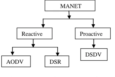
constantly changing topology. While mobile ad hoc networks can be used without a fixed infrastructure, their use is also being considered as part of the vision for a truly ubiquitous communications environment e.g., Wireless Internet. The future success of ad hoc networking will depend on its ability to support existing and future Internet applications and protocols. Such a dynamic environment poses tremendous protocol design challenges at every layer of the network architecture, ranging from physical layer issues to distributed medium access control to routing. Several factors will affect the overall performance of any protocol operating in an ad hoc network. For example, node mobility may cause link failures, which will negatively impact routing and quality-of-service support. Network size, control overhead, and traffic intensity will have a considerable impact on network scalability. These factors along with inherent characteristics of ad hoc networks may result in unpredictable variations in the overall network performance. In the future, MANETs are expected to be deployed in myriads of scenarios having complex node mobility and connectivity dynamics. For example, in a MANET on a battlefield, the movement of the soldiers will be influenced by the commander. In a city-wide MANET, the node movement is restricted by obstacles or maps. The node mobility characteristics are very application specific. Widely varying mobility characteristics are expected to have a significant impact on the performance of the routing protocols like DSR [2], DSDV [3] and AODV [4]. We try to investigate the node mobility effect taking three different scenarios and try to judge its impact and to choose the right protocol so, it might be useful for network designing purpose. MANET routing protocols are subdivided into two categories as shown below:
[image:1.595.316.507.588.716.2]
Fig 1: MANET and its concerned routing protocols.
2.
ROUTING PROTOCOL
Proactive protocols: This type of protocols attempt to find and maintain consistent, up-to-date routes between all
MANET
Reactive Proactive
AODV DSR
destination pairs regardless of the use or need of such routes and we need periodic control messages to maintain routes up to date for each nodes [5]. DSDV is a proactive protocol. Reactive protocols: Routes are created only when a source node request them. Data forwarding is accomplished according to two main techniques: I) Source routing, II) Hop-by-hop routing [5]. DSR, AODV, and TORA are reactive protocols.
2.1 Destination sequenced distance vector
(DSDV)
DSDV is a hop-by-hop protocol in which every node in the network maintains a routing table. A routing table has all of the possible destinations nodes and the number of hops to each destination. Each entry in the routing table has a sequence number assigned by the destination node, implies the freshness of that route, thereby avoiding the formation of routing loops. By periodically update messages, routing tables maintain consistence [6]. Limitation of this routing protocol is that it doesn’t support multipath routing, difficult to determine a time delay for the advertisement of routes [10].
2.2 Dynamic source routing (DSR):
DSR is a source routing protocols, and requires the sender to know the complete route to destination. It is based on two main processes: (a) the route discovery process which is based on flooding and is used to dynamically discover new routes, maintain them in nodes cache, (b) the route maintenance process, periodically detects and notifies networks topology changes. Discovered routes will be cashed in the relative nodes [6]. Here route are stored in memory and data packet contains source route in packet header [11].
3. RELATED WORK
As mobility pattern affects the performance of ad hoc network routing protocols, in this section, we will provide a review on mobility models.
[image:2.595.310.548.580.693.2]Mobility models proposed for ad hoc networks can generally be classified into two groups: entity mobility model and group mobility model [7]. Entity mobility models such as Random Waypoint Mobility (RWP) model attempt to mimic the movement of individual nodes. In this model, each mobile node chooses a random destination and moves towards it with a randomly selected speed which is uniformly distributed in [Vmin, Vmax]. After reaching the destination, the node stops for a duration, and then repeats the whole process again. While entity models assume all nodes move independently, most group mobility models assume that MNs are not completely independent. A general group mobility model, Reference Point Group Mobility (RPGM) model, assumes a group of nodes always move together [8]. In this model, the path of a group is pre-defined by a series of checkpoints, and all the nodes in a group follow the movement of the logical reference center of the group. Every node has its own pre-defined reference point that is displaced around the logical center. Another group mobility model, called the Reference Velocity Group Mobility model [9], is an extension of Reference Point Group Mobility model. In this model, each member node in a group has a velocity that is deviated slightly from the mean group velocity. Analogous to the RPGM model, the mean group velocity serves as a reference velocity for the nodes in the group. This velocity-based group representation is the time derivative of the displacement-based group representation in the RPGM model. The advantage of this mobility model is that a clearer characterization of network partitioning is provided. The mobile nodes are scattered without clear grouping at the beginning with the
network as one large physical cluster. Over time, the nodes move in several directions and are finally separated into a number of smaller groups. However, this model over-simplified the movement of nodes by having the velocity of a node deviates slightly from the mean group velocity. In reality, the velocity of each individual may change arbitrarily within the same group. The characteristic of velocity similarity of every individual is only presented during longer period time instead of instant, so this model could not reflect the scenarios of group mobility in practical deployment of ad hoc networks.
4. TOOL USED FOR SIMULATION
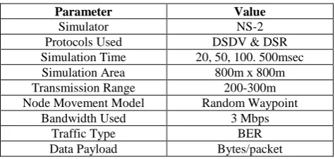
The simulation of these protocols has been carried out using NS-2 simulator on a ―Intel (R) Dual Core CPU T4400 @ 2.20 GHz /RAM-1.96 GB, 1.19 GHz /HDD- 220GB computer and ―Window XP operating system. The network simulator is NS-2 version 2.27 have been taken for analysis the simulation result. NS-2 is an object-oriented simulator written in C++ and OTcl. The simulator supports a 28 class hierarchy in C++ and a similar class hierarchy within the OTcl interpreter. There is a one-to-one interpreted hierarchy and one in the compile hierarchy. The reason to use two different programming languages is that OTcl is suitable for the programs and configurations that demand frequent and fast change while C++ is suitable for the programs that have high demand in speed. NS-2 is highly extensible. It not only supports most commonly used IP protocols but also allows the users to extend or implement their own protocols. It also provides powerful trace functionalities, which are very important in our project since various information need to be logged for analysis. The full source code of NS-2 can be downloaded and compiled for multiple platforms such as UNIX, Windows and Cygwin. NS-2 is chosen as the simulation tool among the others simulation tools because NS-2 supports networking research and education. Ns-2 is suitable for designing new protocols, comparing different protocols and traffic evaluations. NS-2 is developed as a collaborativeenvironment. It is distributed freely and open source..This increase the confidence in it. Simulation have been done efficiently to get the result with less error and proves to be useful for future use. The simulations have been done with different mobility period so, it has been repeated many times to minimize the error level for scenario. The modal parameters that have been used in the following experiments are summarized in Table 1 below:Table 1. Simulation parameters Parameter Value
Simulator NS-2
Protocols Used DSDV & DSR Simulation Time 20, 50, 100. 500msec
Simulation Area 800m x 800m
Transmission Range 200-300m
Node Movement Model Random Waypoint
Bandwidth Used 3 Mbps
Traffic Type BER
Data Payload Bytes/packet
another random destination is chosen after that pause time the pause time is taken for this simulation is vary for 5s, 10s and 5s. This process repeats throughout the simulation, causing continuous changes in the topology of the underlying network. Different network scenario for 10 number of nodes and pause time are generated.
5. METHODOLOGY
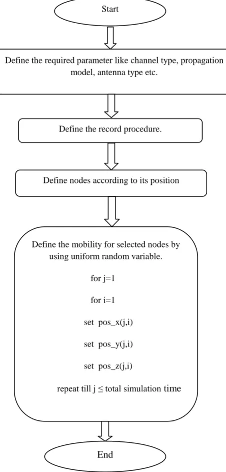
The flow chart show the flow of programming that has been done in NS-2 for source node movement, destination node movement is shown in figure (1), (2) and (3) below:
Fig 2: Flow chart for source node movement
[image:3.595.316.553.78.557.2]Figure (2) and figure (3) shows the methodology that it follows in the network for source node movement and destination node movement. For source node movement the value of node i and j is set to be 1 and the value of node i and j for destination node movement is 1 and N.
Fig 3: Flow chart for destination node movement
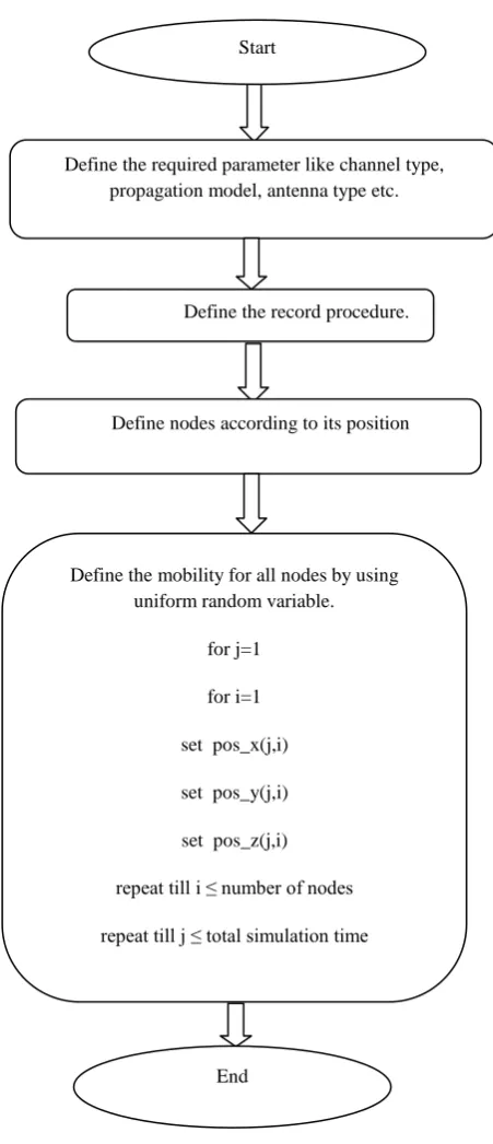
The figure (4) shown below is for all node movement in the network here the value of node i and j is 1but, repeat till i ≤ number of nodes. The flow chart shows the complete description of node movement for all considered scenarios. The overall scenario depend upon this flow chart and initial position is defined according to user in program but when desired node comes in movement its position is random then in define option of TCL (Tool Command Language) file we define the parameters like channel type, propagation model, antenna type etc.Record procedure is used to recall the event after some defined time after that according to user the position of node is define. Now, define the mobility for selected nodes in every scenario using uniform random variable. Here ‘j’ defines the mobility period of movable node the value of j is increases up to total simulation time and this value is multiplied with movable time and ‘i’ defines the nodes number choosen for movement according to user. The Define the required parameter like channel type, propagation
model, antenna type etc.
Define the record procedure.
Define nodes according to its position
Define the mobility for selected nodes by using uniform random variable. for j=1
for i=1 set pos_x(j,i) set pos_y(j,i) set pos_z(j,i)
repeat till j ≤ total simulation time
Start
Define the required parameter like channel type, propagation model, antenna type etc.
Define the record procedure.
Define nodes according to its position
Define the mobility for selected nodes by using uniform random variable.
for j=1 for i=N set pos_x(j,i) set pos_y(j,i) set pos_z(j,i)
repeat till j ≤ total simulation time
Start
End
[image:3.595.46.273.205.677.2]‘x’ , ‘y’ and ‘z’ is random variable and the command set pos is used for random movement of nodes.
[image:4.595.317.559.92.270.2]Fig 4: Flow chart for impact of all node movement
This process is repeated until the value of ‘j’ is equal to or less than the total simulation time. Finally, the program comes to an end. The same procedure is used for the destination and all node movement. The simulation has been done N number of times to get the efficient result at every instant of time. The version used for taking out the simulation result is ns 2.27 and effort has been made to get the best result. The simulation results proves to be good for network designing when the node is source node, destination node also when all nodes is in movement in the network.
[image:4.595.54.280.96.620.2]6.
SIMULATION RESULT & SCENARIO
Fig 5: Screenshot of 10 nodes of DSDV & DSR for source node movement NAM (Network Animator).
Fig 6: Changed position of source node for DSDV &DSR
Fig 7: Packet generated for DSDV & DSR
The X-axis denotes the mobility period in millisecond and Y-axis denotes the packet generated in above figure (7). The blue line indicates the DSDV and green line indicates the Define the required parameter like channel type,
propagation model, antenna type etc.
Define the record procedure.
Define nodes according to its position
Define the mobility for all nodes by using uniform random variable.
for j=1 for i=1 set pos_x(j,i) set pos_y(j,i) set pos_z(j,i) repeat till i ≤ number of nodes repeat till j ≤ total simulation time
End Start
Source Node [0]
Transmission range
Changed position of source Node [0]
Mobility period (msec)
P
ac
k
et
Ge
n
era
[image:4.595.316.565.325.506.2] [image:4.595.306.558.546.702.2]DSR routing protocol. The below figure has been defined in the same manner.
[image:5.595.44.263.121.280.2]Fig 8: Packet loss for DSDV & DSR
Fig 9: Average end to end delay for DSDV & DSR
[image:5.595.38.273.265.487.2]Fig 10: Throughput for DSDV & DSR
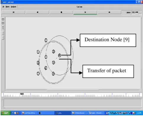
[image:5.595.315.557.306.501.2]Fig 11: Screenshot of 10 nodes of DSDV & DSR for destination node movement.
Fig 12: Changed position of destination node for DSDV &DSR
Fig 13: Packet generated for DSDV & DSR
Destination Node [9]
Position changed of destination Node [9]
Transfer of packet
Mobility period (msec)
Mobility period (msec)
Mobility period (msec) Mobility period (msec)
P
ac
k
et
Ge
n
era
ted
P
ac
k
et
Lo
ss
Av
g
.
E2
E
De
lay
(m
se
c)
Th
ro
u
g
h
p
u
t
(%
[image:5.595.305.544.556.715.2] [image:5.595.39.276.561.717.2]Fig 14: Packet loss for DSDV & DSR
Fig 15: Average end to end delay for DSDV & DSR
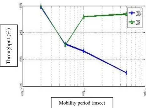
[image:6.595.38.276.316.509.2]Fig 16: Throughput for DSDV & DSR
Fig 17: Screenshot of 10 nodes of DSDV & DSR for all node movement NAM
Fig 18: Packet generated for DSDV & DSR
Fig 19: Packet loss for DSDV & DSR
Movement in all complete 10 Nodes
Mobility period (msec)
Mobility period (msec) Mobility period (msec)
Mobility period (msec) Mobility period (msec)
P
ac
k
et
Ge
n
era
ted
P
ac
k
et
Lo
ss
P
ac
k
et
Lo
ss
Av
g
.
E2
E
De
lay
(m
se
c)
Th
ro
u
g
h
p
u
t
(%
[image:6.595.301.540.329.502.2] [image:6.595.41.275.576.750.2] [image:6.595.303.538.587.743.2]Fig 20: Average end to end delay for DSDV & DSR
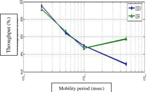
Fig 21: Throughput for DSDV & DSR
7. CONCLUSION
For source node movement DSDV completely dominates DSR routing protocol as DSR is nearly zero throughout the simulation time. For destination node movement the throughput of DSR routing protocol increases as compared to DSDV routing protocol with increase in simulation time. Finally, for all node movement in the network DSR performance is efficient than DSDV routing protocol and the performance of DSDV completely degrades with increase in simulation time under such scenario.
8. ACKNOWLEDGEMENTS
Our special thanks to Dr. S.C. Gupta, Emeritus Professor IIT, Roorkee for his support and guidance.
9. REFERENCES
[1] M.S. Corson, J.P.Macker and G.H. Cirincione, “Internet-based mobile ad hoc networking’. IEEE Internet Computing , Vol. 3, No. 4, pp. 63-70, July/August 1999. [2] D. B. Johnson, D. A. Maltz, and J. Broch, “”DSR: The
dynamic source routing protocol for multi-hop wireless ad hoc networks”,” in Ad Hoc Networking, C. Perkins, Ed. Addison-Wesley, pp. 139–172, 2001.
[3] C. E. Perkins and P. Bhagwat, “Highly dynamic destination sequenced distance vector routing (DSDV) for mobile computers,” in ACM SIGCOMM, 1994, pp. 234–244, 1994.
[4] C. Perkins, “Ad hoc on demand distance vector (AODV) routing, internet draft, draft-ietf-manet-aodv-00.txt.” [5] D. Sun, H. Man, "TCP Flow-based Performance
Analysis of Two On-Demand Routing Protocols for Mobile Ad Hoc Networks", , In Vehicular Technology Conference VTC, 2001, Fall. IEEE VTS 54th, volume 1, pages 272-275, 2001.
[6] J. Broach, D.A. Maltz, D.B. Johnson, Y.C. Hu, and J.Jetcheva, "A Performance Comparison of Multi-Hop Wireless Ad Hoc Network Routing Protocols", Proceedings of the 5th Annual ACM/IEEE International Conference on Mobile Computing, Dallas, TX, October 1998.
[7] T. Camp, J. Boleng, and V. Davies, "A Survey of Mobility Models for Ad Hoc Network Research," Wireless Communication & Mobile Computing (WCMC),Special issue on Mobile Ad Hoc Networking: Research, Trends and Applications, vol.2, no.5, pp.483-502, 2002.
[8] X. Hong, M. Gerla, G. Pei, and C. Chiang, "A group mobility model for ad hoc wireless networks," Proceedings of the ACM International Workshop on Modeling and Simulation of Wireless and Mobile Systems (MSWiM), August 1999.
[9] Karen Wang and Baochun Li, "Group Mobility and Partition Prediction in Wireless Ad-hoc Networks," Proceedings of IEEE International Conference on Communications (ICC 2002), Vol. 2, pp. 1017-1021, New York City, New York, 2002.
[10] Vijayalakshmi M, Avinash Patel, Linganagouda Kulkarnai, “ Qos Parameter Analysis on AODV and DSDV Protocols in Wireless Network”, Vol. 1, pp. 286. [11] Aditi Kumari, Neha Gandotra, Shrikant Upadhyay,
Pankaj Joshi, “Impact of Node Movement on MANET Using Different Routing Protocol for Qos Improvement Under Different Scenario”, International Journal of Smart Sensor and Ad-Hoc Network (IJSSAN), Vol. 1, pp. 95, 2012.
Mobility period (msec)
Mobility period (msec)
Av
g
.
E2
E
De
lay
(m
se
c)
Th
ro
u
g
h
p
u
t
(%
[image:7.595.37.279.325.475.2]