R E S E A R C H
Open Access
An extended data envelopment analysis
for the decision-making
Xiao-Li Meng
1,2and Fu-Gui Shi
1,2**Correspondence: [email protected] 1School of Mathematics and Statistics, Beijing Institute of Technology, Beijing, 100081, China 2Beijing Key Laboratory on MCAACI, Beijing Institute of Technology, Beijing, 100081, China
Abstract
Based on the CCR model, we propose an extended data envelopment analysis to evaluate the efficiency of decision making units with historical input and output data. The contributions of the work are threefold. First, the input and output data of the evaluated decision making unit are variable over time, and time series method is used to analyze and predict the data. Second, there are many sample decision making units, which are divided into several ordered sample standards in terms of production strategy, and the constraint condition consists of one of the sample standards. Furthermore, the efficiency is illustrated by considering the efficiency relationship between the evaluated decision making unit and sample decision making units from constraint condition. Third, to reduce the computation complexity, we introduce an algorithm based on the binary search tree in the model to choose the sample standard that has similar behavior with the evaluated decision making unit. Finally, we provide two numerical examples to illustrate the proposed model.
Keywords: data envelopment analysis; sample standards; time series analysis; binary search tree; decision-making
1 Introduction
In conventional data envelopment analysis (DEA) models, such as CCR model named after Charnes et al. [] and BCC model proposed by Banker et al. [], the inputs and outputs are assumed to be precise. In addition, the constraint condition consists of the evaluated decision making units (DMUs).
In practical studies, the input and output data of the evaluated DMUs are frequently vari-able over multiple time periods (time series data), and it is important to analyze the change of efficiency over time. For example, in the evaluation of travel agencies, transportation, ticket price, accommodation, and labor are always regarded as the inputs, whereas profits and satisfaction of tourists are the outputs. The inputs and outputs are affected by var-ious influential factors, such as the tourism policy, investment of infrastructure, level of starred hotel, annual per-capita income, and level of economic development. However, since the influential factors are variable over time, the inputs, outputs, and efficiencies of travel agencies are variable over time accordingly. Given the current upsurge in interest in DEA, it is surprising that the dynamic DEA attracts very little attention. The only methods we know of this area are Malmquist Productivity Index (MPI) and window analysis. MPI was originally proposed by Caves et al. [] to estimate changes in the overall productivity growth of each DMU over a two-year period by calculating the efficiency value. To deal
with the productivity changes of DMUs over time, Färe et al. [] constructed a DEA-based MPI by combining the efficiency measurement of Farrell [] with the productivity mea-surement of Caves et al. Window analysis, proposed by Charnes et al. [], is adopted to overcome the constraint of limited DMUs and is a benefit to detect the tendency of DMUs over long period with large inputs and outputs. Since then, some improved approaches on the DEA-based MPI or window analysis have been proposed [–]. However, both the DEA-based MPI and window analysis models suffer from one shortcoming: they neglect predicting efficiency of the evaluated DMU.
In many practical evaluation problems, efficiency of every evaluated DMU in a particular period may not be contrasted with the evaluated DMUs, but rather with sample standards determined by manufacturing parameters. The purpose of the contrast is not only to eval-uate efficiency, but also to locate the standard with which the evaleval-uated DMU has similar behavior. For instance, there are many grade standards for the evaluation of travel agencies. Travel agencies from the same region can be evaluated by the same standards separately, and those from different regions should not be evaluated by the same standards because of regional disparities. The standards should be formulated by the regional parameters. Taking outbound tourism as an example, it is an important part for travel agency business in developed regions, but it may not be contained in the travel agency business in some de-veloping regions. Clearly, it is unreasonable that the outbound tourism is included in input measures to evaluate the travel agencies from different regions, and then grade standards in different regions should be formulated in terms of different manufacturing parameters. With these preparations, we then could use different standards to evaluate the level of travel agencies. However, in the existing DEA models, the constraint condition consists of the evaluated DMUs. Furthermore, we categorize DEA models into two types. The first type is the DEA models where the DMU under evaluation is included in the constraint condition [–]. The second type is the DEA models where the DMU under evaluation is not included in the constraint condition. For example, Andersen and Petersen [] de-veloped the superefficiency DEA model, which is identical to the BCC model, except that the DMU under evaluation is not included in the constraint condition. Superefficiency DEA model has been fully explored and applied [–].
Without such considerations, scholars will not be tempted to invest the effort in an-alyzing and predicting the development trend of the DMUs by contrasting with grade standards. In fact, managers can analyze and predict the development trend of input and output data based on historical data and then determine the level by contrasting with sample standards. Furthermore, to maximize profit and ensure proper resource alloca-tion management, efforts can be made through improving influential factors. Therefore, it is a scenario that is worth considering in this case.
2 Preliminaries
2.1 CCR model
As a most frequently used DEA model, the CCR model (Charnes et al. []) supposes that there arenDMUs and that each DMU consumes the same input type and produces the same output type. Letmandsbe the numbers of inputs and outputs, respectively. All inputs and outputs are assumed to be positive. The multiple inputs and multiple outputs of each DMU are aggregated into a single virtual input and a single virtual output. The efficiency of the evaluated DMU is obtained as a ratio of its virtual output to its virtual input subject to the condition in which the ratio of each DMU is not greater than . The corresponding model is as follows:
(CCR) ⎧ ⎪ ⎪ ⎪ ⎪ ⎪ ⎪ ⎪ ⎪ ⎪ ⎪ ⎪ ⎨ ⎪ ⎪ ⎪ ⎪ ⎪ ⎪ ⎪ ⎪ ⎪ ⎪ ⎪ ⎩
maxu,vu
Ty
vTx
,
subject to
uTyj
vTx
j ≤,
j= , . . . ,j, . . . ,n,
v≥, v= ,
u≥, u= ,
()
wherexj= (xj, . . . ,xmj)Tandyj= (yj, . . . ,ysj)T are the input and output vectors of thejth
DMU, DMUjis the evaluated DMU, anduandvare the weight column vectors of outputs and inputs, respectively. The constraint condition consists of all the evaluated DMUs. By applying the Charnes-Cooper transformation (Charnes and Cooper []) in the model (), the following equivalent linear model is obtained:
(PCCR)
⎧ ⎪ ⎪ ⎪ ⎪ ⎪ ⎪ ⎪ ⎪ ⎪ ⎪ ⎪ ⎪ ⎪ ⎪ ⎨ ⎪ ⎪ ⎪ ⎪ ⎪ ⎪ ⎪ ⎪ ⎪ ⎪ ⎪ ⎪ ⎪ ⎪ ⎩
maxμμTy,
subject to
wTxj–μTyj≥,
j= , . . . ,j, . . . ,n,
wTx= ,
w≥,
μ≥, μ= .
()
The optimal objective values of models () and () fall into the range of (, ]. The rela-tionship between DEA efficiency and the optimal objective value (Cooper et al. []) can be obtained as follows.
Definition (DEA efficient) If the optimal objective value of the evaluated DMU is equal
to and there is at least one optimal solution in which the optimal weight vectors of inputs and outputs are greater than , then the evaluated DMU is DEA efficient.
Definition (weak DEA efficient) If the optimal objective value of the evaluated DMU is
Definition (DEA inefficient) If the optimal objective value of the evaluated DMU is less than , then the evaluated DMU is DEA inefficient.
2.2 Time series method
A discrete ordered set of observed data that changes over time is called a time series and denoted asy(t) ={y(t),y(t), . . . ,y(ti), . . .}, wherey(ti) is the observed data at the momentti. Time series can be divided into nonparametric and parametric models. The nonparamet-ric model estimates the covariance or the spectrum without assuming that the process has a particular structure. By contrast, the parametric model assumes that the underlying sta-tionary stochastic process has a certain structure. The time series model is used to extract meaningful statistic and other characteristics of the observed data and then to predict the development trend. It is usually composed of three parts, namely,
Y(t) =f(t) +p(t) +X(t), ()
wheref(t) is the trend term, which reflects the changing trend ofY(t),p(t) is the periodic term, reflecting the cyclical change ofY(t), andX(t) is the stochastic term, which reflects the influence of random factors ofY(t). Here we assume thatX(t) is a normal stationary stochastic process (Chatfield [], Gershenfeld []).
3 An extended DEA model
In this section, based on the fundamental CCR model,we propose an extended DEA model. In the model, the input and output data of the evaluated DMUs are predicted by the time series method based on the historical data. The constraint condition consists of one of the sample standards determined by the production strategy. There are many sam-ple DMUs, which are further divided into several ordered samsam-ple standards in terms of manufacturing parameters. Moreover, sample DMUs in the same standard have similar behavior. It is important to stress here that the evaluated DMU does not belong to the set of sample DMUs. The extended DEA model is as follows:
⎧ ⎪ ⎪ ⎪ ⎪ ⎪ ⎪ ⎪ ⎪ ⎪ ⎪ ⎪ ⎨ ⎪ ⎪ ⎪ ⎪ ⎪ ⎪ ⎪ ⎪ ⎪ ⎪ ⎪ ⎩
maxu,vu
Ty E(t)
vTx
E(t), subject to
uT¯ykh(s)
vTx¯
kh(s) ≤,
k= , . . . ,m¯, h= , . . . ,nk¯ ,
v≥, v= ,
u≥, u= ,
()
where xE(t) and yE(t) are the input and output vectors of the evaluated DMU at the
momentt, every element of xE(t) andyE(t) is nonnegative, andx¯kh(s) andy¯kh(s), which
is
⎧ ⎪ ⎪ ⎪ ⎪ ⎪ ⎪ ⎪ ⎪ ⎪ ⎪ ⎪ ⎪ ⎪ ⎪ ⎨ ⎪ ⎪ ⎪ ⎪ ⎪ ⎪ ⎪ ⎪ ⎪ ⎪ ⎪ ⎪ ⎪ ⎪ ⎩
maxμμTyE(t),
subject to
wTxkh¯ (s) –μTykh¯ (s)≥,
k= , . . . ,m¯, h= , . . . ,nk¯ ,
wTx
E(t) = ,
w≥, w= ,
μ≥, μ= .
()
It is easy to see that the evaluated DMU is not contained in the constraint condition. The optimal objective values of uTyE(t)
vTx
E(t) andμ
TyE(t) in models () and () vary in (, +∞). The
superefficiency definition of the proposed model is given as follows.
Definition (DEA superefficient) An evaluated DMU is DEA superefficient if its optimal
objective value is higher than and there is at least one optimal solution in which the optimal weight vectors of inputs and outputs are greater than .
To determine the efficiency of the evaluated DMUs in the proposed model, the follow-ing theorems are given by considerfollow-ing the relationship between DEA efficiency and the optimal objective value.
Theorem If the evaluated DMU is DEA superefficient by the kth standard,then the
optimal objective value is greater than.
Theorem The evaluated DMU is DEA efficient by all the combinations of sample DMUs
in the kth standard if and only if there exists an optimal objective value that is equal to
and the optimal weight vectors of inputs and outputs are greater than.
Theorem The evaluated DMU is weak DEA efficient by the kth standard if and only if
the optimal objective value is equal toand there does not exist any optimal solution in
which the optimal weight vectors of inputs and outputs are greater than.
Theorem The evaluated DMU is DEA inefficient by all the combinations of sample
DMUs in the kth standard if and only if all optimal objective values are less than.
4 The relationship between DEA efficiency and the production frontier
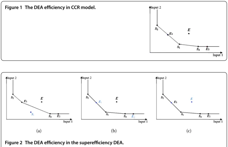
Figure 1 The DEA efficiency in CCR model.
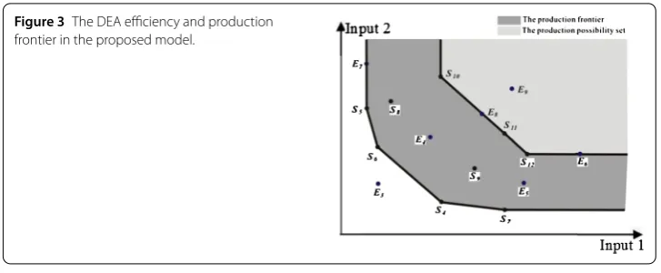
[image:6.595.116.479.81.315.2](a) (b) (c)
Figure 2 The DEA efficiency in the superefficiency DEA.
4.1 DEA efficiency and the production frontier in the conventional DEA models
In the CCR model, the constraint condition consists of all the DMUs, and the production frontier is spanned by efficient DMUs and weak efficient DMUs. As shown in Figure , the production frontier is spanned by DMUsS,S,S,E, andE. DMUsS,S,S, andEare DEA efficient, DMUEis weak DEA efficient, and DMUEis DEA inefficient.
In the superefficiency model, the constraint condition consists of all the DMUs ex-cept the evaluated DMU, and the production frontier is spanned by all the corresponding DMUs without the DMU under evaluation. If the evaluated DMU is located on the weak production frontier, then it is weak efficient (Yu et al. [], Wei et al. []). If the evaluated DMU is located on the efficient production frontier, then it is efficient (that is, there exist positive optimal weight vectors of inputs and outputs such that the efficiency of the eval-uated DMU is equal to the efficiency of a certain sample DMUs and the optimal objective value is equal to (Doyle and Green [], Salo and Punkka []). If the evaluated DMU is located in the production possibility set but is not located on the production frontier, then it is inefficient. Otherwise, the evaluated DMU is superefficient. For example, the evalu-ated DMUSis superefficient in Figure (a), the evaluated DMUsEandEare efficient and weak efficient, respectively, in Figure (b), and the evaluated DMUEis inefficient in Figure (c).
4.2 DEA efficiency and the production frontier in the proposed model
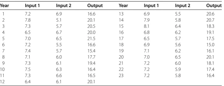
Unlike conventional DEA models, in the proposed model, the constraint condition con-sists of one of the sample standards, and the production frontier is spanned by different combinations of sample DMUs from the constraint condition. To illustrate this, now we suppose that there are seven evaluated DMUsE-Eand that thekth standard is the con-straint condition consisting of nine sample DMUsS-S.
Figure 3The DEA efficiency and production frontier in the proposed model.
sample DMUsS-S, the least efficient production frontier is spanned by sample DMUs
S-S, and the other production frontiers that are spanned by different combinations of sample DMUsS-Sare located between the most and least efficient production frontiers. The evaluated DMUE is closer to the coordinate origin than the most efficient pro-duction frontier, and then the efficiency of DMUEis higher than that of every sample DMU from the constraint condition. In such a case, the constraint condition consists of all sample DMUs of thekth standard, the optimal objective value is greater than , and the evaluated DMUEis DEA superefficient.
If the evaluated DMU is located between the most and least efficient production fron-tiers, then there is at least one optimal objective value equal to for the evaluated DMU, such as DMUE,E,E,E, andE. Clearly, in Figure , it is easy to see that DMUEis DEA superefficient by the least efficient production frontierS-Sand DEA inefficient by the most efficient production frontierS-S; then DMUEis DEA efficient (i.e., the
opti-mal objective value of the evaluated DMUEis equal to , and the optimal weight vectors
of inputs and outputs are greater than ) by a combination of thekth standard. Similarly, there is an optimal objective value of DMUEequal to , and the optimal weight vectors
of inputs and outputs are greater than . In the following, we consider the evaluated DMU
E, which is weak DEA efficient relative to the least efficient production frontier, and then there is an optimal objective value of the DMUEequal to . A similar analysis applies to the evaluated DMUE; we can see that there is also an optimal objective value equal to . Finally, we take the evaluated DMUEinto account, it can be expressed by a linear combination of DMUSandS, and thus it is DEA efficient by the least efficient produc-tion frontier, and there is an optimal objective value equal to . The evaluated DMUEis located in the production possibility set of the least efficient production frontier but not located on the least efficient production frontier. Then DMUE is DEA inefficient, and the optimal objective value is less than . In fact, in the proposed model, the determined production frontier is spanned by the difference between the production possibility sets of the most and least efficient production frontiers.
5 Algorithm
to determine the sample standard with which the evaluated DMU has similar behavior. If the evaluated DMU is superefficient by thetth standard, then the constraint condition should turn to the standard with higher efficiency. If the evaluated DMU is weak efficient or inefficient by thetth standard, then the constraint condition should turn to the standard with lower efficiency. Otherwise, the evaluated DMU is located in thetth standard, that is, the evaluated DMU has similar behavior with thetth standard. Let [x] denote the greatest integer not greater thanx. The algorithm is summarized as follows.
Step: Star with dividing the sample DMUs intom¯ ordered sample standards. Lett= ,
t=m.¯
Step: Use thetth andtth standards to evaluate the evaluated DMU.
If the evaluated DMU is DEA efficient by thetth (ortth) standard, then Stop - the evaluated DMU has similar behavior with thetth (ortth) standard;
If the evaluated DMU is DEA superefficient (or inefficient) by thetth and thetth standard, then
Stop - the evaluated DMU has not similar behavior with all the sample standards;
Else
Turn to Step .
Step: If the evaluated DMU is DEA superefficient by thetth standard and inefficient by
thetth standard, then
t←[(t+t)/]
If the evaluated DMU is DEA inefficient by thetth standard, then t←t; Turn to Step ;
If the evaluated DMU is DEA superefficient by thetth standard, then
t←t; Turn to Step ;
Else
Turn to Step .
If the evaluated DMU is DEA superefficient by thetth standard and weak efficient by thetth standard, then
Stop - the evaluated DMU has similar behavior with the(t– )th standard. If the evaluated DMU is DEA inefficient by thetth standard and superefficient by
thetth standard, then
t←[(t+t)/]
If the evaluated DMU is DEA superefficient by thetth standard, then
t←t; Turn to Step ;
If the evaluated DMU is DEA inefficient by thetth standard, then
t←t; Turn to Step ;
Else
Turn to Step .
If the evaluated DMU is DEA weak efficient by thetth standard and superefficient by thetth standard, then
Table 1 Production status in the last 23 years
Year Input 1 Input 2 Output Year Input 1 Input 2 Output
1 7.2 6.9 16.6 13 6.9 5.5 20.6
2 7.8 5.1 20.1 14 7.9 5.8 20.7
3 7.3 5.7 20.5 15 8.1 6.4 18.3
4 6.5 6.7 20.0 16 6.8 6.2 19.1
5 7.0 6.5 21.5 17 6.5 5.7 17.5
6 7.2 5.5 16.6 18 6.9 5.6 15.0
7 7.4 5.7 15.4 19 7.1 6.2 16.1
8 7.1 6.0 17.7 20 7.0 6.5 20.1
9 7.3 6.1 19.4 21 7.2 6.0 18.1
10 7.5 6.3 16.4 22 7.2 5.9 17.4
11 7.3 6.6 16.5 23 7.2 5.8 16.4
12 6.4 6.1 20.1
6 Illustrative examples
In this section, we present two numerical examples to illustrate the proposed model. For simplicity, “sample DMU” will be abbreviated to “SDMU”.
6.1 The first example
In this example, the data of the evaluated DMU in the last years are provided in Table . There are sample DMUs with two inputs and a single output listed in Table , and the sample DMUs SDMUi, SDMUi, and SDMUi (i= , , , , ) are located in theith
standard. By the proposed model the production status of the evaluated DMU in the th year is analyzed.
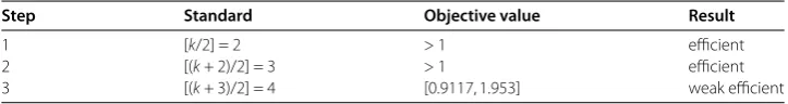
Firstly, time series method is used to analyze the inputs and outputs. In Figure , all thep
values oft-statistics are less than ., and then the original hypothesis whose parameter is should be rejected, and the three unknown parameters are considered to be significant. The AR() model is suitable for fitting the Input sequence, and the predicting equation is as follows:
x(t) = . + .x(t– ) – .x(t– ).
Similarly, the predicting equations of Input and Output are given respectively by
x(t) = . – .x(t– ),
y(t) = . – .y(t– ).
The DEA model is as follows:
⎧ ⎪ ⎪ ⎪ ⎪ ⎪ ⎪ ⎪ ⎪ ⎪ ⎪ ⎪ ⎪ ⎪ ⎪ ⎨ ⎪ ⎪ ⎪ ⎪ ⎪ ⎪ ⎪ ⎪ ⎪ ⎪ ⎪ ⎪ ⎪ ⎪ ⎩
maxμμT[. – .y(t– )],
subject to
wTxkh¯ –μTykh¯ ≥,
k= , . . . , ; h= , , ,
w[. + .x(t– ) – .x(t– )]
+w[. – .x(t– )] = ,
w≥, w= ; μ≥, μ= .
Figure 4 Maximum likelihood estimation of Input 1.
Table 3 The processes of evaluation
Step Standard Objective value Result
1 [k/2] = 2 > 1 efficient
2 [(k+ 2)/2] = 3 > 1 efficient
3 [(k+ 3)/2] = 4 [0.9117, 1.953] weak efficient
Secondly, the production status of the evaluated DMU in the th year is evaluated by the sample standards. Since the outputs of the constraint condition are interval values, it is impossible to calculate every value. Then the two endpoints of interval are defined as the pessimistic and optimistic values separately (Wang et al. []). For example,ais the pes-simistic value, andbis the optimistic value in the interval (a,b] or [a,b]. Since all the points of an interval lie between the endpoints (i.e., the pessimistic and optimistic values), it is reasonable that the interval values are replaced by the pessimistic and optimistic values. Each sample DMU in the constraint condition is divided into two corresponding sample DMUs based on the pessimistic and optimistic values. The process is given in Table , and the evaluated DMU is located in the fourth sample standard in the next year.
6.2 The second example
Strategic groups are always used in the strategic management of insurance companies, and groups companies have similar business models or similar combinations of strategies. An insurance company can ascertain major competitors, obtain the competitive situation, and then formulate production strategy by analyzing strategic groups [].
.. Dividing the sample insurance companies into ordered strategic groups
In this example, we only study the property insurance companies. The Appendix gives the overall production status of sample property insurance companies from to by the averaging method (the data is collected from Yearbooks of China’s Insurance). We assume that the formation of strategic groups is determined according to the following five manufacturing parameters: total number of employees (TNE), fixed assets (FA), sales tax and extra charges (STEC), earned insurance premiums (EIP), and expenses of payments (EP). The first three manufacturing parameters are inputs, and the others are outputs. FA, STEC, EIP, and EP are described in the unit of million Yuan RMB. As shown in Table , the sample DMUs are divided into six standards (i.e., six sample strategic groups).
.. Predicting production status of Samsung Fire & Marine Insurance(China)
Company Ltd
[image:11.595.117.479.168.216.2]Table 4 Six strategic groups (from low to high)
Standard Property Insurance Companies
1 Bohai Property Insurance Company Limited; Chang an Property and liability Insurance Limited; Du-bang Property & Casualty Insurance Company Limited; Nipponkoa Insurance Company (China) Limited; China Continent Insurance; Ancheng Property & Casualty Insurance Company Limited.
2 Sinosafe Insurance Company Limited; Da Zhong Insurance Company Limited; Ming An Property & Casualty Insurance Company Limited; China Huanong Property & Casualty Insurance Company Limited; Liberty Insurance Company Limited.
3 Huatai Insurance Company of China, Limited; Aioi Insurance Company Limited; American Chubb Group of Insurance; Bank of China Insurance Company Limited; Zurish Insurance, Beijing; Alltrust Insurance Company Limited.
4 China Life Property & Casualty Insurance Company Limited; Tianan Property Insurance Company Limited; Dinghe Insurance; Sun Alliance Insurance Company; Generali China Insurance Company Limited; Sompo Japan Insurance (China) Company Limited.
5 The Tokio Marine & Nichido Fire Insurance Company (China) Limited; Anxin Agricultural Insurance Company Limited; AIG General Insurance Company China Limited; Allianz Insurance Company Guangzhou Branch; Hyundai Insurance (China) Company Limited.
[image:12.595.118.479.341.427.2]6 Mitsui Sumitomo Insurance (China) Company Limited; Guoyuan Agricultural Insurance Company; China Export & Credit Insurance Corporation; Sunlight Mutual Insurance Company.
Table 5 The production status of Samsung F&M from 2008-2014
Year TNE FA STEC EIP EP
2008 62 1.67 2.28 65.78 55.68
2009 75 2.25 2.95 92.22 81.66
2010 91 2.43 9.2 87.94 68.42
2011 138 9.16 13.75 125.03 233.71
2012 192 10.01 19.88 134.23 102.67
2013 226 17.52 24.8 142.87 247.14
2014 325 19.27 28.1 195.56 217.11
Table 6 The predicted production status in 2014
2014 TNE FA STEC EIP EP
Predicted 286 20.03 29.8 174.2 232.5
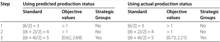
Table 7 The evaluation processes and results
Step Using predicted production status Using actual production status
Standard Objective values
Strategic Groups
Standard Objective values
Strategic Groups
1 [6/2] = 3 > 1 No [6/2] = 3 > 1 No
2 [(6 + 2)/2] = 4 > 1 No [(6 + 2)/2] = 4 > 1 No
3 [(6 + 4)/2] = 5 [0.62, 2.69] Yes [(6 + 4)/2] = 5 [0.73, 2.21] Yes
.. Evaluating the production efficiency by the sample strategic groups
[image:12.595.114.478.472.500.2] [image:12.595.117.478.545.615.2]7 Conclusions
In the conventional DEA model, the inputs and outputs are known exactly, and the con-straint condition consists of the evaluated DMUs. However, in many real applications, the observed data of the evaluated DMUs are variable over time. The efficiency of every evalu-ated DMU in a particular period may not be contrasted with the evaluevalu-ated DMUs, but with sample standards determined by production strategy. Moreover, the development trend of the evaluated DMU, which is an important index to the budgetary decision-making and management system, is often required to be predicted.
Appendix
Table 8 The overall production status of sample property insurance companies. Unit: Person; RMB1000000
Property Insurance Companies TNE FA STEC EIP EP
Bank of China Insurance Company Limited 2,532 491.15 179.04 2,568.46 1,289.60
Aioi Insurance Company Limited 81 2.94 2.12 50.08 21.61
Ancheng Property & Casualty Insurance Company Limited
2,607 131.70 87.62 1,462.89 865.90
Allianz Insurance Company Guangzhou Branch
120 2.38 23.17 98.29 125.06
Anxin Agricultural Insurance Company Limited
362 171.66 25.61 637.41 378.86
Bohai Property Insurance Company Limited 3,254 242.34 85.02 1,268.91 822.27 China Continent Insurance 34,719 1,282.01 487.41 13,105.77 4,838.26 Da Zhong Insurance Company Limited 1,971 101.92 88.73 1,322.05 923.86
Dinghe Insurance 869 54.78 63.13 890.89 492.32
The Tokio Marine & Nichido Fire Insurance Company (China) Limited
280 9.30 23.02 402.39 207.36
Du-bang Property & Casualty Insurance Company Limited
8,663 599.14 104.56 3,378.89 1,070.38
China Life Property & Casualty Insurance Company Limited
14,576 690.25 1,023.03 14,584.57 8,087.69
Guoyuan Agricultural Insurance Company 1,023 50.97 13.90 1,428.10 954.51 Sinosafe Insurance Company Limited 5,835 1,167.15 286.24 4,370.28 2,043.66 China Huanong Property & Casualty
Insurance Company Limited
370 10.86 14.85 230.85 136.24
Huatai Insurance Company of China, Limited
4,128 147.70 229.09 3,251.63 1,882.15
Liberty Insurance Company Limited 632 20.37 29.26 439.49 263.19
AIG General Insurance Company China Limited
931 9.27 27.98 749.04 281.25
Ming An Property & Casualty Insurance Company Limited
3,854 70.40 106.16 1,556.03 923.78
American Chubb Group of Insurance 122 4.14 7.25 99.86 49.87
Sompo Japan Insurance (China) Company Limited
307 9.78 12.71 296.89 166.82
Nipponkoa Insurance Company (China) Limited
47 1.85 1.72 23.67 13.97
Mitsui Sumitomo Insurance (China) Company Limited
319 4.84 22.23 567.87 333.88
Zurish Insurance, Beijing 74 1.35 13.10 70.46 41.40
Sun Alliance Insurance Company 94 2.44 8.05 95.44 56.85
Tianan Property Insurance Company Limited
14,084 221.65 453.61 6,870.18 4,848.25
Hyundai Insurance (China) Company Limited
53 4.14 4.76 57.60 78.41
Sunlight Mutual Insurance Company 2,170 102.14 16.71 1,846.27 1,283.38 Alltrust Insurance Company Limited 4,964 93.89 292.19 3,812.56 2,636.82 Chang an Property and liability Insurance
Limited
3,316 139.71 93.77 1,276.34 876.85
China Export & Credit Insurance Corporation
2,159 395.69 38.97 4,101.75 4,958.59
Generali China Insurance Company Limited 137 5.05 10.33 144.06 61.92
Competing interests
Authors’ contributions
Both authors contributed equally and significantly in writing this paper. Both authors read and approved the final manuscript.
Authors’ information
This work is supported by the National Natural Science Foundation of China (11371002) and Specialized Research Fund for the Doctoral Program of Higher Education (20131101110048).
Publisher’s Note
Springer Nature remains neutral with regard to jurisdictional claims in published maps and institutional affiliations.
Received: 22 June 2017 Accepted: 6 September 2017 References
1. Charnes, A, Cooper, WW, Rhodes, E: Measuring the efficiency of decision making units. Eur. J. Oper. Res.2, 429-444 (1978)
2. Banker, RD, Charnes, A, Cooper, WW: Some models for estimating technical and scale inefficiencies in data envelopment analysis. Manag. Sci.30, 1078-1092 (1984)
3. Caves, DW, Christensen, LR, Diewert, WE: The economic theory of index numbers and the measurement of input, output, and productivity. Econometrica50, 1393-1414 (1982)
4. Färe, R, Grosskopf, S, Lindgren, B, Roos, P: Productivity change in Swedish pharmacies 1980-1989: a nonparametric Malmquist approach. J. Product. Anal.3, 85-102 (1992)
5. Farrell, MJ: The measurement of productivity efficiency. J. R. Stat. Soc. A120, 253-281 (1957)
6. Charnes, A, Clark, CT, Cooper, WW, Golany, B: A developmental study of data envelopment analysis in measuring the efficiency of maintenance units in the U.S. air forces. Ann. Oper. Res.2, 95-112 (1985)
7. Chen, Y, Alib, AI: DEA Malmquist productivity measure: new insights with an application to computer industry. Eur. J. Oper. Res.159, 239-249 (2004)
8. Chung, SH, Lee, AHI, Kang, HY, Lai, CW: A DEA window analysis on the product family mix selection for a semiconductor fabricator. Expert Syst. Appl.35, 379-388 (2008)
9. Kazley, AS, Ozcan, YA: Electronic medical record use and efficiency: a DEA and windows analysis of hospitals. Socio-Econ. Plan. Sci.43, 209-216 (2009)
10. Halkos, GE, Tzeremes, NG: Exploring the existence of Kuznets curve in countries’ environmental efficiency using DEA window analysis. Ecol. Econ.68, 2168-2176 (2009)
11. Yang, HH, Chang, CY: Using DEA window analysis to measure efficiencies of Taiwan’s integrated telecommunication firms. Telecommun. Policy33, 98-108 (2009)
12. Kao, A: Malmquist productivity index based on common-weights DEA: the case of Taiwan forests after reorganization. Omega38, 484-491 (2010)
13. Wang, YM, Lan, YX: Measuring Malmquist productivity index: a new approach based on double frontiers data envelopment analysis. Math. Comput. Model.54, 2760-2771 (2011)
14. Zhang, N, Choi, Y: Total-factor carbon emission performance of fossil fuel power plants in China: a metafrontier non-radial Malmquist index analysis. Energy Econ.40, 549-559 (2013)
15. Horta, IM, Camanho, AS: A nonparametric methodology for evaluating convergence in a multi-input multi-output setting. Eur. J. Oper. Res.246, 554-561 (2015)
16. Meng, XL, Shi, FG: An extended inequality approach for evaluating decision making units with a single output. J. Inequal. Appl.2017, 199 (2017)
17. Meng, XL, Shi, FG: A generalized fuzzy data envelopment analysis with restricted fuzzy sets and determined constraint condition. J. Intell. Fuzzy Syst.33, 1895-1905 (2017)
18. Kao, A, Liu, ST: Fuzzy efficiency measures in data envelopment analysis. Fuzzy Sets Syst.113, 427-437 (2000) 19. Entani, T, Maeda, Y, Tanaka, H: Dual models of interval DEA and its extension to interval data. Eur. J. Oper. Res.136,
32-45 (2002)
20. Lertworasirikul, S, Fang, SC, Joines, JA, Nuttle, HL: Fuzzy data envelopment analysis (DEA): a possibility approach. Fuzzy Sets Syst.139, 379-394 (2003)
21. Ruggiero, J: Impact assessment of input omission on DEA. Int. J. Inf. Technol. Decis. Mak.4, 359-368 (2005) 22. Wang, YM, Greatbanks, R, Yang, JB: Interval efficiency assessment using data envelopment analysis. Fuzzy Sets Syst.
153, 347-370 (2005)
23. Cooper, WW, Ruiz, JL, Sirvent, I: Choosing weights from alternative optimal solutions of dual multiplier models in DEA. Eur. J. Oper. Res.180, 443-458 (2007)
24. Düzakin, E, Düzakin, H: Measuring the performance of manufacturing firms with super slacks based model of data envelopment analysis: an application of 500 major industrial enterprises in Turkey. Eur. J. Oper. Res.182, 1412-1432 (2007)
25. Podinovski, VV: Computation of efficient targets in DEA models with production trade-offs and weight restrictions. Eur. J. Oper. Res.181, 586-591 (2007)
26. Liu, ST, Chuang, M: Fuzzy efficiency measures in fuzzy DEA/AR with application to university libraries. Expert Syst. Appl.36, 1105-1113 (2009)
27. Wei, QL, Chang, TS: DEA-type models for designing optimal systems and determining optimal budgets. Math. Comput. Model.54, 2645-2658 (2011)
28. Yang, A, Wu, DD, Liang, L, Liam, O: Competition strategy and efficiency evaluation for decision making units with fixed-sum outputs. Eur. J. Oper. Res.212, 560-569 (2011)
30. Bian, YW, Hu, M, Xu, H: Measuring efficiencies of parallel systems with shared inputs/outputs using data envelopment analysis. Kybernetes44, 336-352 (2015)
31. Fukuyama, H, Shiraz, RK: Cost-effectiveness measures on convex and nonconvex technologies. Eur. J. Oper. Res.246, 307-319 (2015)
32. Hadi-Vencheh, A, Hatami-Marbini, Z, Ghelej, B, Gholami, K: An inverse optimization model for imprecise data envelopment analysis. Optimization64, 2441-2454 (2015)
33. Mehdiloozad, M, Mirdehghan, SM, Sahoo, BK, Roshdi, I: On the identification of the global reference set in data envelopment analysis. Eur. J. Oper. Res.245, 779-788 (2015)
34. Shabani, A, Torabipour, SM, Saen, RF, Khodakarami, M: Distinctive data envelopment analysis model for evaluating global environment performance. Appl. Math. Model.39, 4385-4404 (2015)
35. Yang, M, Li, YJ, Liang, L: A generalized equilibrium efficient frontier data envelopment analysis approach for evaluating DMUs with fixed-sum outputs. Eur. J. Oper. Res.246, 209-217 (2015)
36. Zanella, A, Camanho, AS, Dias, TG: Undesirable outputs and weighting schemes in composite indicators based on data envelopment analysis. Eur. J. Oper. Res.245, 517-530 (2015)
37. Aleskerov, F, Petrushchenko, V: DEA by sequential exclusion of alternatives in heterogeneous samples. Int. J. Inf. Technol. Decis. Mak.15, 5-22 (2016)
38. Mardani, A, Zavadskas, EK, Streimikiene, D, Jusoh, A, Khoshnoudi, M: A comprehensive review of data envelopment analysis (DEA) approach in energy efficiency. Renew. Sustain. Energy Rev.70, 1298-1322 (2017)
39. Meng, XL, Shi, FG: An extended DEA with more general fuzzy data based upon the centroid formula. J. Intell. Fuzzy Syst.33, 457-465 (2017)
40. Andersen, P, Petersen, NC: A procedure for ranking efficient units in data envelopment analysis. Manag. Sci.39, 1261-1264 (1993)
41. Lee, HS, Chu, CW, Zhu, J: Super-efficiency DEA in the presence of in-feasibility. Eur. J. Oper. Res.212, 141-147 (2011) 42. Lee, HS, Zhu, J: Super-efficiency infeasibility and zero data in DEA. Eur. J. Oper. Res.216, 429-433 (2012)
43. Banker, RD, Chang, H, Zheng, Z: On the use of super-efficiency procedures for ranking efficient units and identifying outliers. Ann. Oper. Res.116, 1-15 (2015)
44. Li, Y, Xie, J, Wang, M, Liang, L: Super efficiency evaluation using a common platform on a cooperative game. Eur. J. Oper. Res.255, 884-892 (2016)
45. Charnes, A, Cooper, WW: Programming with linear fractional functionals. Nav. Res. Logist.9, 181-186 (1962) 46. Cooper, WW, Seiford, LM, Zhu, J: Handbook on Data Envelopment Analysis, pp. 1-227. Kluwer Academic, Boston
(2004)
47. Chatfield, C: The Analysis of Time Series: an Introduction, 6th edn. Chapman & Hall, Boca Raton (2016)
48. Gershenfeld, N: In: The Nature of Mathematical Modeling, pp. 205-208. Cambridge University Press, New York (1999) 49. Yu, A, Wei, QL, Brockett, P, Zhou, L: Construction of all DEA efficient surfaces of the production possibility set under
the generalized data envelopment analysis model. Eur. J. Oper. Res.95, 491-510 (1996)
50. Wei, QL, Yan, H, Hao, G: Characteristics and construction method of surface and weak surface of DEA production possibility, Hong Kong Polytechnic University, Research Report of Department of Management, May (2000) 51. Doyle, J, Green, R: Efficiency and cross-efficiency in DEA: derivations, meanings and uses. J. Oper. Res. Soc.45,
567-578 (1994)
52. Salo, A, Punkka, A: Ranking intervals and dominance relations for ratio-based efficiency analysis. Manag. Sci.57, 200-214 (2011)
53. Dulá, JH: An algorithm for data envelopment analysis (DEA), School of Business, University of Mississippi, University, MS 38677 (1998)