Quantitative Strategy Based on Decision Tree and Bollinger Band

2019 International Conference on Applied Mathematics, Modeling, Simulation and Optimization (AMMSO 2019) ISBN: 978-1-60595-631-2

Quantitative Strategy Based on Decision Tree and Bollinger Band

Ke WANG, Zhong-yan LI, Tian-yang SONG and Zi-yang ZHANG

School of Mathematics and Physics, North China Electric Power University, Beijing 102206

Keywords: Quantitative investment, Decision tree, Bollinger bands, Wavelet analysis.

Abstract. Because stock investors often invest blindly and emotionally, and the quantitative investment strategy is more rational and reliable, so the purpose of this paper is to establish a suitable quantitative strategy for investors. We selected six indicators as stock price forecasting indicators, constructed the model by using CART algorithm, Mallat algorithm and Brin Belt index.The test results show that the earnings gap of the multi-short portfolio of the modified model is significantly increased, reaching the level of 3%. Combining with the timing strategy of Brin Belt, the total earnings can exceed the average earnings of technology stocks by 3.3%.

Introduction

In recent years, more investors have paid attention to the concept of quantitative trading. Stock selection[1] is a process in which investors use their own analytical methods to select target investment products from all tradable varieties.

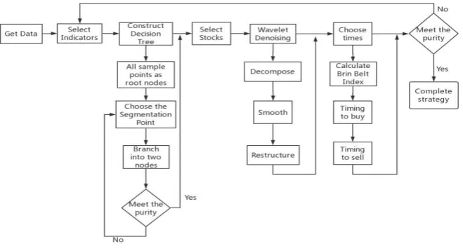
This paper uses decision tree model to select stocks with long-term investment value.And the wavelet denoising method[2] is used to denoise the financial time series. Finally we use the Brin Belt index to select the time.

Figure 1. Technology Roadmap.

Construct Quantitative Strategies

Decision tree model stock selection method combines the advantages of multi-factor linear model[3] and black box model[4,5]. The limitation of model linear hypothesis is relaxed, and the understandability and visualization of the model are ensured. There are two main steps in the construction of decision tree: the selection of classification attributes and the pruning of decision tree branches.

Stock Index Selection

After choosing the indicators, the technology stocks are selected as an example of the application of CART model. And we have revised the indicators as follows:

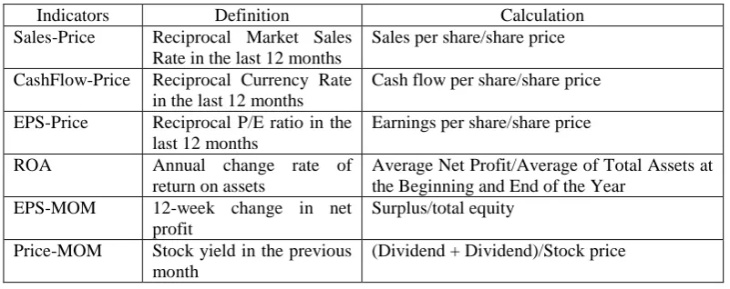
Table 1. Key Indicators of Decision Tree Classification.

Indicators Definition Calculation

Sales-Price Reciprocal Market Sales

Rate in the last 12 months

Sales per share/share price

CashFlow-Price Reciprocal Currency Rate

in the last 12 months

Cash flow per share/share price

EPS-Price Reciprocal P/E ratio in the

last 12 months

Earnings per share/share price

ROA Annual change rate of

return on assets

Average Net Profit/Average of Total Assets at the Beginning and End of the Year

EPS-MOM 12-week change in net

profit

Surplus/total equity

Price-MOM Stock yield in the previous

month

(Dividend + Dividend)/Stock price

CART Algorithm

We choose the CART algorithm of classification and regression tree as the basic method of decision tree and the starting point of a series of research.

We construct dynamic tree CART model based on historical data of science and technology stocks.

We calculate the monthly relative return on each stock by subtracting the median of the total stock return for the month. In this way, we labeled the monthly samples as winning (1) and losing (-1). Then, we record the rate of return on the winning and losing samples over the next month as a long and short combination.

We construct dynamic tree CART model based on historical data of science and technology stocks.

Step1. Establish static decision tree based on sample data from 2012 to 2015;

Step2. The January 2016 sample data are fed into the decision tree model obtained in step 1 for classification. Based on the classification, the stocks are classified into multi-empty portfolios, and their returns in February 2016 are recorded.

Step3. Establish a decision tree based on the sample data from early 2012 to January 2016, and send the February 2016 sample data into the model for prediction. Establish a multi-empty portfolio to record its earnings in March 2016;

Step4. Roll these steps in turn until October 2017.

Using the method of dynamic decision tree, we classify the out-of-sample data and form a monthly multi-empty combination. By averaging the monthly multiple short portfolio profit margin, we get that the dynamic decision tree model wins the short portfolio 0.93% on average from the beginning of 2012 to the end of October 2017. Considering the transaction cost and impact cost, we think that the excess return of the model is not very significant. So, we need to prune the decision tree.

Pruning Method

Because of the problem of pre-pruning learning algorithm, post-pruning algorithm is widely used. This method is the result of deleting one or more subtrees of the original tree. In the pruning process, some subtrees are deleted by replacing them with some leaf nodes. The proportion of training instances belonging to this category is marked on the corresponding leaves.

Figure 2. Pre-pruning of Static Decision Tree.

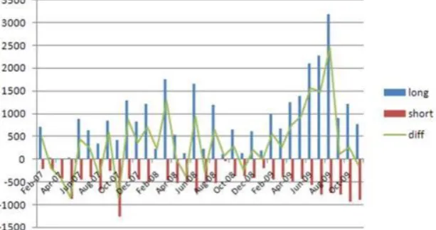
Ultimately, we build a dynamic decision tree and make a long short term portfolio. With the passage of time, the dynamic decision tree becomes more and more effective. The stock classification is more effective through the dynamic model, and stocks whose earnings characteristics are not significantly predicted will not be invested in long or short portfolios, but will be discarded directly.

Figure 3. Number comparison of multi-short portfolio stocks.

In terms of quantity, the total number of long and short portfolios selected is only less than half of the total sample, which reduces the problem of too many classified samples caused by simple decision tree, and the number of stocks in long and short portfolios is gradually stable.

Denoising by Wavelet Analysis

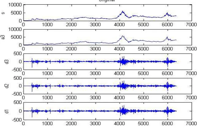
SymN wavelet performs well in continuity, support length, filter length and so on, and it has very good symmetry, that is to say, it can reduce the phase distortion when analyzing and reconstructing signals to a certain extent.

Time series are decomposed[7], denoised and reconstructed[8] by Sym2 wavelet.

Figure 5. Reconstructed Time Series Image.

Timing of Brin Belt

Firstly, the average and standard deviation of stock price time series[9] are calculated. The positive and negative standard deviations of the medium track are set to the upper and lower tracks respectively, which are expressed by the following formula:

Std = Standev(Close,Length) Midline = Xaverage(Close,Length) Lowline = Midline-2Std

Uppline = Midline+2Std

Brin bandwidth is defined as: StdMidRatio = StdMidLine

TrendIndex is the difference between the average bandwidth of the upper and lower Brin belts, which can be used to indicate the magnitude of price fluctuations. Namely:

TrendIndex=Average(Uppline,N)-Average(Lowline,N) UppBand=Higest(TrendIndex,N)

LowBand=lowest(TrendIndex,N)

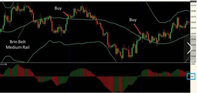
When the stock index fluctuates, TrendIndex is also in a narrowing range. If there is a clear breakthrough in price up or down, it means that there has been a rising or falling trend. At this time, the stock can be bought or sold.

The long trading rules are as follows:

1. K-line must break the Brin Belt Medium Rail and be above it.

2. An Awesome oscillator corresponding to a green bar with a level higher than 0. 3. Place a stop order higher than the K-line low of 2 points.

4. Place the stop at least two points below the nearest low.

Figure 6. Multi-Diagram.

Short trading rules are as follows:

1. K line must break the middle track of Brin belt and be below it.

2. An Awesome oscillator corresponding to a red bar with a level below 0. 3. Place a stop-sale order below the K-line low of 2 points.

4. Place the stop at least two points above the nearest high point.

5. The profit target is aimed at the low level or 2-3 times the risk in the transaction. For example, if you run a risk of 10 points, the target is 20 to 30 points of profit.

Figure 7. Short Diagram.

After the decision tree selection, combined with the Brin Belt timing strategy, the total earnings can exceed the average earnings of technology stocks by 3.3%.Revenue retrospective return curve as shown in Fig.8.

Figure 8. Revenue Backtracking Profit Curve.

Conclusions

the level of 3%. Combining with Brin Belt timing strategy, the total return can exceed the average return of technology stocks by 3.3%. In terms of the number of stock options, the multi-short portfolio is less than half of the total sample, which effectively reduces the difficulty of stock selection and reflects the accuracy of classification. Therefore, it is a complete and practical quantitative timing strategy.

Acknowledgement

This research was financially supported by the National Natural Science Foundation of China (Grant No. 11571107).

References

[1] C. Chang, J. Lin. LIBSVM[J]. ACM Transactions on Intelligent Systems and Technology (TIST), 2011(3): 32-43.

[2] S.G. Mihov, R.M. Ivanov, A.N. Popov. Denoising Speech Signals by Wavelet Transform[J]. Annual Journal of Electronics, 2009: 238-284.

[3] E.F. Fa Ma, K.R. French. Multifactor Explanations of Asset Pricing Anomalies[J].The Journal of Finance, 1996(1): 51-55.

[4] K. Park, H. Shin. Stock price prediction based on a complex interrelation network of economic factors[J]. Engineering Applications of Artificial Intelligence, 2013(5-6): 12-16.

[5] C. Li, S. Xu, W. Wang, W. Li. Stock Prediction on Basis of General Regression Neural Network Optimized with Modified Simple Particle Swarm Optimization[J]. EN, 2012(16): 324-335.

[6] M. Baker, L. Litov, J.A. Wachter, J. Wurgler. Can Mutual Fund Managers Pick Stocks? Evidence from Their Trades Prior to Earnings Announcements[J]. The Journal of Finance, 2010(3): 165-178.

[7] S.G. Mihov, R.M. Ivanov, A.N. Popov. Denoising Speech Signals by Wavelet Transform[J]. Annual Journal Of Electronics, 2009: 238-284.

[8] I. Daubechies. The wavelet transform, time-frequency localization and signal analysis[J]. IEEE Transactions on Information Theory, 1990(1): 43-55.