2019 2nd International Conference on Informatics, Control and Automation (ICA 2019) ISBN: 978-1-60595-637-4
Comparative Study of Unconstrained Mechanical Optimization Methods
Based on Two-variable Rosenbrock Function
Chun-ming LI
1,2and Xiao-li YIN
1,2,*1
College of Mechanical and Electrical Engineering, China University of Petroleum (East China), Qingdao 266580, China
2
Shengli College, China University of Petroleum (East China), Dongying 257061, China
*Corresponding author
Keywords: Optimization algorithm, multi-dimensional unconstrained optimization, unimodal
assumption, programming verification, Rosenbrock Canyon.
Abstract. The unconstrained optimization method (UOM) plays an important role in the field of physics, mathematics, statistics, etc. Rosenbrock function is a 4-degree function with a curved canyon. It is most suitable for testing UOM. However, the test hasn't done. We have written 14 UOM computer programs, 12 of which contain our new algorithm. From the optimal result, the 2-order approximation direction is the best, followed by the conjugate direction, followed by the negative gradient direction. For quadratic fitting function method, linear fitting gradient method and unbounded polyhedron deformation method, a new algorithm for moving points was proposed. When the new point is better than all of the other points, the other points should close up to it. And when the new point is worse than all of the other points, it should close up to the best point or center point. The improvement of moving points makes these optimization directions be effective for complex objective functions.
Introduction
Any algorithm for finding global extreme point or optimal parameters can be called optimization methods. It belongs to the field of applied mathematics and computational mathematics. The optimization problem exists in other fields too, such as classical continuum physics, theoretical, mathematical & computational physics, particle and nuclear physics, physical chemistry, pure mathematics, mathematical physics, fluid dynamics, actuarial science, applied information economics, astrostatistics, biostatistics, business statistics, mechanical, etc. The research on optimization method not only needs the algorithm innovation, but also needs the computer program verification. Instead of relying on computational software, we write computer programs and validate algorithms in time. Among the research of related projects, we haven't found any reference on UOM comparative study.
Rosenbrock function is a 4-degree non-convex function, introduced by Howard H. Rosenbrock in
1960[1], which is known as Rosenbrock Canyon or Banana function. It can test algorithms.
In this paper, a computer program is compiled to test all optimization methods with the same objective function. On the basis of classical optimization methods, we have made the following improvements and innovations:
1) One-dimensional blindwalking optimization method[2].
2) The obtaining conjugate directions method based on geometric relations[3].
3) The obtaining conjugate direction method based on auxiliary direction[4].
4) Three-search method to obtain conjugate direction based on negative gradient direction[5].
5) Multidimensional quadratic fitting function method[6].
6) Linear fitting gradient method[6].
7) Constructing conjugate direction method. Powell method is the most classical optimization
method. Three improvements is based on it[7].
8) Improved unbounded polyhedron deformation method(simplex and complex method) [8].
9) Second-order approximate direction method(Newton direction method)[2].
10) The improved second-order approximate fixed-point method based on the idea of blind path
finding[9].
11) An improved negative gradient direction method based on the idea of blind path finding[10].
12) The algorithm of moving new points (for the first time in this paper).
Rosenbrock Function
Two-dimensional Rosenbrock function is following.
2 2
2
2 1 1
3
1 2 1 1
2
2 1
2
1 2 1
f
1
min f 100 1
400 400 2 2
f
200 200
1200 400 2 400
400 200
x x x
x x x x
x x
x x x
x
x
x
x
H
(1)
The global minimum point is
1 1 . It is difficult to find the descent direction pointing to the Textremum point in Rosenbrock Canyon. It can only be approached by small step ceaselessly and circuitously. When a certain section bottom of Canyon is meeted, even if a better descent direction is found, it can only go forward by micro step. If the termination condition value is too large, or the scope of the search direction is limited, it is difficult to approach the extremum point.
The Adaptive Coordinate Descent Method
The optimal point whose objective function value is less than 10-10 can be found after 325 times of
objective function calculation[11]. This process is not reproduced by writing computer program.
The Negative Gradient Direction Method and Three Newton Methods
The optimal pointxk1 at the directions k is obtained by 1D optimization method[2]. The sawtooth
phenomenon occurs in the algorithm. If the current point is closer to the extremum point, the worse the optimization effect is.
than 1, the fixed-point method(Eq.3) is not suitable. The inverse matrix can be insteaded by its adjugate matrix.
1
f f
k k
s H x (2)
1 1
f f
k k k
x x H x (3)
The initial point is
0.4 0.6
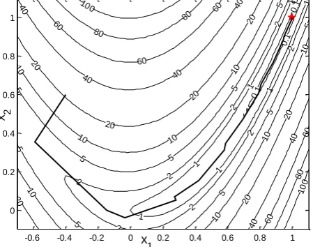
T. The termination condition value is 1.0 10 6. The initial step sizeof one-dimensional blind pathfinding optimization is 0.1. For the negative gradient direction method, the process is the solid line 1 in Fig.1. The computation of blind pathfinding negative gradient
direction method[10] will be smaller. For higher-degree multi-dimensional 2-order approximate
fixed-point method based on the blind pathfinding idea[9], the process is the dash-dot line 2 in Fig.1.
For the classical fixed-point method which is also called as Newton iteration method, the process is the dashed line 3 in Fig.1. For higher-degree multidimensional two-order approximate direction method, the process is the dotted line 4 in Fig.1.
-0.6 -0.4 -0.2 0 0.2 0.4 0.6 0.8 1
[image:3.595.186.410.294.476.2]0 0.2 0.4 0.6 0.8 1 x 1 x 2 0.1 0.1 0.1 1 1 1 1 1 1 1 2 2 2 2 2 2 2 2 5 5 5 5 5 5 5 5 5 5 10 10 10 10 10 10 10 10 20 20 20 20 20 20 20 40 40 40 40 40 40 60 60 60 60 60 80 80 80 100 10 0 1:solid line 3:dashed line 2:dash-dot line 4:dotted line
Figure 1. The negative gradient direction method and three Newton methods.
The Quasi-uniform Coordinate Transformation Method
In order to avoid the zigzag phenomenon, the eccentricity of the objective function is online can be reduced by coordinate transformation. Then a better optimal result can be obtained along the negative gradient direction. For DFP (Davidon, Fletcher, Powell) algorithm, and BFGS (Broyden, Fletcher, Goldfarb, Shanno) algorithm formula, the similar search process is obtained, which is shown in fig.2.
-0.6 -0.4 -0.2 0 0.2 0.4 0.6 0.8 1
0 0.2 0.4 0.6 0.8 1 x1 x 2 0.1 0.1 0.1 1 1 1 1 1 1 1 2 2 2 2 2 2 2 2 5 5 5 5 5 5 5 5 5 5 10 10 10 10 10 10 10 10 20 20 20 20 20 20 20 40 40 40 40 40 40 60 60 60 60 60 80 80 80 100 10 0
[image:3.595.187.412.598.775.2]The Gradient Related Conjugate Direction Methods
For a general objective function, if it is replaced by its second-order approximation at a certain point, then it is the formula (4).
1 T Tf
2 c
x x Gx b x (4)
Where, a real symmetric positive definite matrix G is the two-order partial derivative matrix at the point x. According to the optimization characteristics and the condition of new direction pointing to
the extremum point, after the optimizing along s 0 , the direction s 1 should satisfies Eq.(5).
T
0 1
0
s G s (5)
After the optimal point xk1 is obtained by 1-dimensional optimization along s k starting from
k
x , the conjugate direction sk1 of s k can be obtained from the gradients g k and gk1[3].
If sk1 is in the plane determined by s k , gk1, it can be obtained by undetermined coefficient
method(UCM). For 2-dimensional Rosenbrock function, an optimization round is carried out along the negative gradient direction and its conjugate direction in turn.
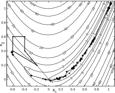
The conjugate direction group method is based on the linear independent vector group (CDM). Figure 3 is the optimization process. The reference [3] and UCM coincides with dashed line 1 and 2. The optimization efficiency of CDM is poor. If the orthogonal vector group changes at each round, the process is shown as solid line 3. If the orthogonal vector group doesn't change, the process is shown as solid line 4.
-0.6 -0.4 -0.2 0 0.2 0.4 0.6 0.8 1
0 0.2 0.4 0.6 0.8 1
x
1 x 2
0.1
0.1 0.1
1
1
1
1
1 1
1
2
2 2
2 2
2
2 2
5
5
5
5 5 5
5
5 5
5
10
10 10
10
10
10 10
10
20
20 20 20
20
20 20
40
40 40
40
40 40
60
60
60
60 60 80
80
80 100
100 1 and 2: dashed line
[image:4.595.200.396.404.558.2]3 and 4:solid line
Figure 3. Three conjugate direction methods.
Two Contiguous Conjugate-direction Methods Based on Auxiliary Direction
For the optimization problem with the objective function (4), the x k and xk1 are optimal points
(the numerical approximate point of the extreme point on this direction) along the direction s j by
1-dimensional optimization starting from different points. The direction s k xk1x k and s j
are conjugative relating to G. After an optimal point is obtained along a direction, another optimal point is obtained along the same direction starting from an auxiliary point outside the above optimization route. The link of two optimal points is regarded as the next optimization direction. The auxiliary point can be gotten at the negative gradient direction of the first optimal point. Along the
negative gradient direction, three-search method is obtained[5].
-0.6 -0.4 -0.2 0 0.2 0.4 0.6 0.8 1 0 0.2 0.4 0.6 0.8 1 x1 x 2 0.1 0.1 0.1 1 1 1 1 1 1 1 2 2 2 2 2 2 2 2 5 5 5 5 5 5 5 5 5 5 10 10 10 10 10 10 10 10 20 20 20 20 20 20 20 40 40 40 40 40 40 60 60 60 60 60 80 80 80 100 10 0
Figure 4. Two conjugate direction methods based on auxiliary direction.
The Multidimensional Quadratic Fitting Function and Linear Fitting Gradient Method
In accordance with the 1-dimensional quadratic fitting function method, according to the objective function value of some points, the quadratic fitting function of the objective function is constructed by the undetermined coefficient method. The extremum point of the fitting function is regarded as the new point. The worst point or the most edge point is removed. Then the new fitting function can be
constructed. So an iterative is completed[6]. In order to avoid multimodal influence, several nearest
points construct the fitting function.
The optimization process is shown as dotted line in Fig. 5. When the parameter reaches the software limit, the error is larger, but the optimal point is still good. It shows that the algorithm has good robustness.
-0.6 -0.4 -0.2 0 0.2 0.4 0.6 0.8 1
0 0.2 0.4 0.6 0.8 1 x1 x 2 0.1 0.1 1 1 1 1 1 1 1 2 2 2 2 2 2 2 2 5 5 5 5 5 5 5 5 5 5 10 10 10 10 10 10 10 10 20 20 20 20 20 20 20 40 40 40 40 40 40 60 60 60 60 60 80 80 80 100 10 0
Figure 5. Two fitting function methods.
The Alternate Coordinate Direction Method and the Improved Powell Method
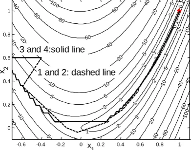
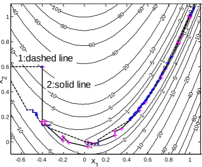
The improved and basic algorithm of classic Powell method is well-known. Reference [7] has improved it. In figure 6, the dashed line 1 in Fig.6 shows the process of the alternate coordinate direction method, and the solid line 2 in Fig. 6 shows the improved Powell method. For the
unbounded polyhedron deformation method, the vertex number is N1. If the new point is by
[image:5.595.199.397.419.579.2]-0.6 -0.4 -0.2 0 0.2 0.4 0.6 0.8 1 0
0.2 0.4 0.6 0.8 1
x
1
x 2
0.1
0.1 0.1
1
1
1
1
1 1
1
2
2 2
2 2
2
2 2
5
5
5
5 5 5
5
5 5
5
10
10 10
10
10
10 10
10
20
20 20 20
20
20 20
40
40 40
40
40 40
60
60
60
60 60 80
80
80 100
10 0
[image:6.595.199.398.70.234.2]2:solid line 1:dashed line
Figure 6. The alternate coordinate direction method and Powell method.
Conclusion
1) the quasi-uniform coordinate transformation method and the conjugate direction are the best. 2) all classic optimization methods with deterministic direction are proposed based on the unimodal assumption in which the objective function is regarded as quadratic function. The change of initial point will not affect the optimization result.
3) since the computer programs have written, the theoretical system can be developed.
Acknowledge
Teaching Reform Research Foundation of Shengli College in China University of Petroleum(East China) [number JG201725], Natural Science Foundation of Shandong Province (CN) [number ZR2018PEE009] and Shandong University of Science and Technology [number J17KA044].
Reference
[1] https://en.wikipedia.org/wiki/Rosenbrock_function. 17 May 2018.
[2] Li Chunming 2010 Blind-walking optimization method Journal of Networks,5(12) 1458-1466.
[3] Liu Qing, Liu Xiao, Yin Xiaoli, Li Chunming 2017 Conjugate method of adjacent directions based
on gradient vector of objective function Journal of Gansu Sciences in China29(5)15-21.
[4] Yin Xiaoli, Sun Feng, Li Chunming. Six search optimization method on obtaining conjugate direction after continuous negative gradient directions[J]. Journal of Frontiers of Computer Science and Technology, [2018-08-29]. http://kns.cnki.net/kcms/detail/
[5] Li Chunming, Zhang Xiaohua, Yin Xiaoli 2017 The program verification of the three-seeking and
six-seeking method based on the conjugate direction. 5th International Conference on Machinery,
Materials and Computing Technology, March 25-26, Beijing, China.
[6] Li Chunming, Wang Haoyu, Xu Wenhui, Li Xu 2017 Multidimensional two-time fitting function
optimization method Journal of Gansu Sciences in China29(5)26-28.
[7] Liu Xiao, Yin Xiaoli, Li Chunming 2019 On the improvement of the Powell optimization method
Chinese Journal of Machine Design36(0) in publish.
[9] LI Chunming, Zhu Mingye, Li Wanteng 2017 Second-order approximation point method based on
the blind walking idea Journal of the China University of Petroleum ( Edition of Natural Science)
41(1) 144-149.
[10] Li Chunming 2016 Negative gradient direction method for blind person exploring the way
Chinese Journal of Gansu Sciences28(5)116-122.
[11] Loshchilov, I., M. Schoenauer, M. Sebag 2011 Adaptive coordinate descent Genetic and