©2008 Royal Statistical Society 0035–9254/08/57149 57,Part2,pp.149–163
Generalized monotonic functional mixed models
with application to modelling normal tissue
complications
Matthew Schipper,
Innovative Analytics, Kalamazoo, USA
Jeremy M. G. Taylor
University of Michigan, Ann Arbor, USA
and Xihong Lin
Harvard School of Public Health, Boston, USA
[Received September 2006. Revised September 2007]
Summary.Normal tissue complications are a common side effect of radiation therapy. They are the consequence of the dose of radiation that is received by the normal tissue surrounding the site of the tumour. Within a specified organ each voxel receives a certain dose of radiation, leading to a distribution of doses over the organ. It is often not known what aspect of the dose distribution drives the presence and severity of the complications. A summary measure of the dose distribution can be obtained by integrating a weighting function of dose (w.d/) over the density of dose. For biological reasons the weight function should be monotonic. We propose a generalized monotonic functional mixed model to study the dose effect on a clinical outcome by estimating this weight function non-parametrically by using splines and subject to the monoto-nicity constraint, while allowing for overdispersion and correlation of multiple obervations within the same subject. We illustrate our method with data from a head and neck cancer study in which the irradiation of the parotid gland results in loss of saliva flow.
Keywords: Dose effect; Functional data; Monotonicity; Non-parametric regression; Normal tissue complications; Overdispersion; Splines
1. Introduction
Radiation therapy is commonly used to treat cancer. The goal is to deliver the highest possible dose to the site of a tumour and the lowest possible dose to the surrounding normal tissue. Higher doses to the tumour result in more damage to the cancer cells, whereas higher doses to the normal tissue cause damage that can lead to normal tissue complications. Pneumonitis is an example of a serious but rare normal tissue complication that is experienced by lung cancer patients. Other examples include rectal failure in colon cancer patients and xerostoma (loss of saliva production) in head and neck cancer patients. There are many potential treatment plans depending on the number, direction and intensity of the radiation beams. In choosing a treat-ment plan, the physician must trade off maximizing damage to the tumour with minimizing damage to the surrounding tissue. To do this efficiently, it is necessary to understand precisely
Address for correspondence: Matthew Schipper, Innovative Analysis, 161 East Michigan Avenue, Kalamazoo, MI 49007, USA.
how the dose of radiation to the normal tissue and the probability or the severity of normal tissue complications are related.
Modern treatment planning techniques allow the physician to compute, for a given treatment plan, the spatial distribution of dose within the tissue being irradiated. This dose distribution is typically represented by using the dose volume histogram (DVH) (Lichter, 1991). It is common for the region of the tumour to be given an approximately uniform dose. Such is not so for the surrounding normal tissue where the dose depends on its proximity to the tumour as well as on the treatment plan.
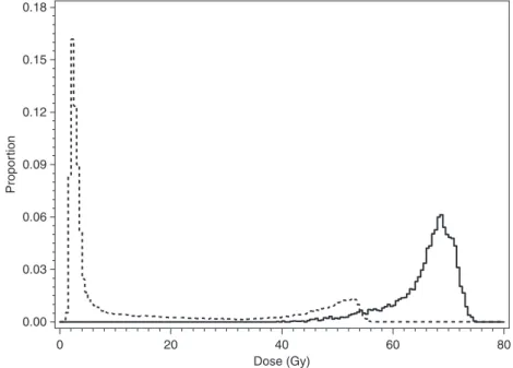
Our motivating example is the head and neck cancer data that were collected at the University of Michigan. This study involved 82 patients with a cancerous tumour in their head or neck who were treated with external beam radiation therapy. A common side effect in these patients is loss of saliva flow due to the irradiation of the parotid glands. The two parotid glands, one in either cheek, are responsible for producing saliva. The doses of radiation to each voxel in the parotid ranged from 0 to 82 Gy and the DVH bin widths are 0.5 Gy. Fig. 1 is an example of the DVHs for the two glands (ipsilateral and contralateral) of a particular subject. For a more detailed description of the data, see Section 4.1. The question of major interest in such settings is how to relate the radiation dose distribution that is received by the normal tissue to the observed complication, e.g. saliva flow. Simple approaches include creating a summary measure of the dose distribution, e.g. the mean dose, and regressing the normal tissue complication on the summary dose measure.
It is of significant interest to estimate the effect of the dose distribution on a normal tissue complication non-parametrically. In other words, we are interested in relating a functional pre-dictor to a scalar outcome. Ramsay and Silverman (1997), chapter 10, considered a functional model that relates a precisely measured functional covariate to a scalar outcome. A more general
0.18
0.15
0.12
0.09
Propor
tion
0.06
0.03
0.00
0 20 40
Dose (Gy)
60 80
model is the functional generalized linear model (James, 2002; Zhanget al., 2007), where the observed functional predictor is assumed to be measured over time and with error. Rather than time, our functional predictor is measured over dose. Denote byp.d/the density of the dose distribution, i.e. the fraction of the organ receiving dose less thancis0cp.d/dd. Then a general measure of the dose effect is given byp.d/w.d/dd, wherew.d/is a weighting function to be estimated. We can easily see that commonly used dose summaries are special cases of this gen-eral summary measure. The mean dose is obtained with a linear weighting function (w.d/=d). The partial volume or proportion of tissue receiving dose greater thanX Gy is obtained by an indicator function (w.d/=I.d > X/).
In this paper, we propose a generalized monotone functional mixed model which relates a multivariate complication outcome to a dose distribution. The dose effect is summarized by using the summary measure that was discussed above. Within this model framework we pro-pose a new method for non-parametric estimation ofw.d/subject to two constraints. The first is that any biologically meaningful estimate ofw.d/should be monotone since increasing dose cannot lead to lower probability or severity of complications. The second is thatw.0/=0. The biological reason for this is clear since zero dose should correspond to no effect. The statistical reason for this constraint is model identifiability. We definew.d/as the integral of a smooth positive function, where the smooth positive function is obtained as a positive transformation of an unconstrained regression spline. Our model differs from the functional generalized lin-ear model in that we wish to estimatew.d/monotonically, and we introduce random effects to accommodate correlation and overdispersion of multivariate complication outcomes. Max-imum likelihood is used for model fitting.
There are many approaches to monotone non-parametric regression (Friedman and Tibshira-ni, 1984; Ramsay, 1988, 1998; Kelly and Rice, 1990; Hall and Huang, 2001; Gelfand and Kuo, 1991; Holmes and Heard, 2003; Dunson, 2005). Existing techniques were generally designed to estimate a monotone relationship between two scalar quantities and hence are not directly applicable to relating a scalar outcome to a functional predictor (dose distribution). Although some of the existing techniques could potentially be modified to this setting, they generally impose monotonicity through constraints on the parameter space. Such constraints complicate estimation and inference with the possibility of estimates on the boundary of the parameter space. In contrast, our proposed method requires no such constraints.
This paper is organized as follows. Section 2 describes the model as well as the formulation of
w.d/. Section 3 discusses estimation of the model. We describe in detail the head and neck cancer saliva data in Section 4 and apply the proposed methods to analyse the saliva data. Section 5 presents simulation results, followed by discussion in Section 6.
2. The generalized monotonic functional mixed model
LetYijdenote the complication outcome for thejth observation.j=1, . . . ,J) of theith subject
.i=1, . . . ,n/. We assume that, conditionally on random effectsbi,Yij follows an exponential
family distribution (McCullagh and Nelder, 1989) with meanμijgiven by
g.μij/=XTijα+
D
0 pij.d/
w.d/dd+ZTijbi .1/
whereg.·/is a link function,αandbirepresent fixed and random effects with corresponding
design matricesXijandZij, andpij.d/is the density of the dose distribution; [0,D] is the range
of dose. We further assume that random effectsbi are independent and each followsN.0,Σ/.
L=n
i=1
J
j=1
f.Yij|bi/f.bi/dbi, .2/
wheref.Yij|bi/is the conditional density ofYij|biandf.bi/is the normal likelihood density of
bi. For the head and neck cancer data, the outcome is saliva flow, which is measured separately
from each subject’s two parotid glands and henceJ=2. Since saliva flows are measured as rates, we assume thatYij|bifollows a Poisson distribution in our analysis. We could alternatively make
a weaker assumption by using the quasi-likelihood with the conditional meanE.Yij|bi/=μij
and the conditional variance var.Yij|bi/=μij(McCullagh and Nelder, 1989; Breslow and
Clay-ton, 1993). The random effectsbiaccount for correlation between bivariate observations within
subject as well as possible overdispersion. Sinceαincludes an intercept term andp.d/is a den-sity function satisfyingp.d/dd=1, we need to constrainw.d/for identifiability. Specifically, ifw.d/is an arbitrary constantw, then
p.d/w.d/dd=w,
which would confound with the interceptα0. We hence constrainw.d/byw.0/=0.
As discussed in Section 1, biologically,w.d/needs to be monotone increasing. A convenient way to impose this constraint is to definew.d/as the integral of a non-negative function. We consider the formulation
w.d/= d
0 s.c/
dc .3/
where
s.d/=h{r.d/} .4/
and
r.d/=L+4
l=1
βlBl.d/: .5/
Hereh.·/is a known, non-negative continuous function defined on the real line, theBl.·/sare
known basis functions which are defined by using Linterior knots, e.g. B-spline bases, and theβlare unknown parameters. In this formulation, equation (5) imposes smoothness whereas equations (3) and (4) impose monotonicity. No constraint is needed for theβs.
It follows that model (1) can be rewritten as
g.μij/=XTijα+
D
0 pij.d/ d
0 h L+4
l=1
βlBl.c/
dcdd+ZTijbi: .6/
In the absence of the functional effectp.d/w.d/dd, model (1) specifies a generalized linear mixed model (Breslow and Clayton, 1993). However, it can be seen from model (6) that, since h.·/can be non-linear, the second term need not be a linear function ofβl. Thus the dose sum-mary measure in model (1) may also not be linear inβland model (6) is a functional extension of the generalized linear mixed model.
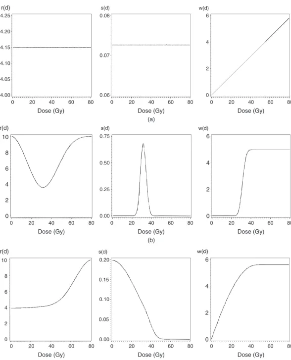
Fig. 2 demonstrates the flexibility of the proposed functional dose summary measurep.d/×
(a)
10
8
6
4
2
0 10
8
6
4
2
0 r(d)
r(d)
0.00 0.05 0.10 0.15 0.20 s(d)
s(d) w(d)
0.00 0.25 0.50 0.75 Dose (Gy)
0 20 40 60 80
Dose (Gy)
0 20 40 60 80
Dose (Gy)
0 20 40 60 80
(b)
Dose (Gy)
0 20 40 60 80
Dose (Gy)
0 20 40 60 80
Dose (Gy)
0 20 40 60 80
(c) Dose (Gy)
0 20 40 60 80
Dose (Gy)
0 20 40 60 80
Dose (Gy)
0 20 40 60 80
r(d)
4.25 0.08 6
4
2
0 0.07
0.06 4.20
4.15
4.10
4.05
4.00
s(d) w(d)
6
4
2
0
6
4
2
0
Fig. 2. Three examples ofw.d/with the correspondingr.d/ands.d/: (a) linear; (b) sigmoidal; (c) plateau
and the saliva flow example, we found that relatively few (two or three) knots worked well. A standard choice for knot placement is to place the knots by using percentiles of the data.
a large constant so as not to restrict the range ofs.d/. Sincer.d/is estimated non-parametri-cally, the estimates ofw.d/are robust to the choice ofh.·/. Our numerical results confirm this. However, if we wish to test the null hypothesis of no dose effect, it is desirable to chooseh.·/so thath.0/=0, e.g.h.z/=z2orh.z/=a{φ.0/−φ.z/}if the normal density is used, whereais an arbitrary scale constant to make the range ofs.d/practically unconstrained. Then no dose effect occurs whenβ1=β2=. . .=βL+4=0 and a likelihood ratio test can be used to test this null
hypothesis. Another special case of our model is whenβ1=β2=. . .=βL+4, which corresponds
to a mean dose model sinceΣLl+4Bl.t/=1 for allt. A likelihood ratio test can also be used to test
whether mean dose is a suitable summary of the dose effect. Using a symmetrich.·/function technically results in non-identifiability of the signs ofr.d/sinceh.z/=h.−z/. In practice this will generally not be an issue and does not affect the estimator ofw.d/.
3. Estimation
The specification of the generalized monotone functional mixed model (1) assumes that the dose distributionp.d/is known and continuous. In practice only the empirical distribution ofp.d/, which is called the DVH, is observed. The DVH discretizes dose intoK bins and measures the proportion of the gland that received a dose within each bin. Fig. 1 shows two example DVHs of the saliva data of a representative subject.
Using the DVH as an empirical estimate ofp.d/, we replace model (1) by
g.μij/=XTijα+ K
k=1
pij.dk/w.dk/+ZijTbi .7/
whereKis the number of DVH bins,dk=.k−1/bin width, i.e.dkis the left end point of thekth
bin andp.dk/is the proportion of normal tissue receiving dose in bink. We also approximate
the integral in equation (3) asw.d1/=0 and
w.dk/≈ k
l=2
s.dl/Δd
fork=2, . . . ,K, whereΔdis the bin width. Plugging this into model (7), we obtain
g.μij/=XTijα+ K
k=2
pij.dk/
k
m=2
s.dm/Δd
+ZT
ijbi
=XTijα+K
k=2
pij.dk/
k
m=2
h L+4
l=1
βlBl.dm/
Δd +ZTijbi: .8/
Estimation in this model proceeds with the maximum likelihood method which maximizes the likelihood function (2), where the conditional likelihood ofL.Yij|bi/is specified by using the
mean model (8) under the exponential family. The random effectsbiare assumed to beN.0,Σ/.
In contrast with the generalized linear mixed model (Breslow and Clayton, 1993), where regres-sion coefficients enter the linear predictor linearly, regresregres-sion coefficientsβls in model (8) enter
g.μij/non-linearly. The marginal likelihood (2) generally does not have a closed form
4. Application to head and neck cancer data
4.1. Description of the data
In this section we fit the generalized monotone functional mixed model to the head and neck cancer data that were introduced in Section 1. Patients with a cancerous tumour in their head or neck were treated with external beam radiation therapy. A common side effect in these patients is loss of saliva flow due to the irradiation of the parotid glands. The parotid glands, of which there are two, one in either cheek, are responsible for producing saliva. The doses of radiation to each voxel in the parotid ranged from 0 to 82 Gy and the DVH bin widths are 0.5 Gy; thus K=164. Fig. 1 is an example of the DVHs for the two glands of a particular subject. Clearly one gland of this subject received a much larger dose than the other. This is common because in treatment planning the dose to the gland on the opposite side from the tumour (contralateral) is usually minimized, whereas no such attempt is made for the gland on the same side as the tumour (ipsilateral). Saliva flows are measured separately from both cheeks. We study in this paper the effect of the dose distribution on saliva flow at 6 months after the baseline. This analysis involved 157 saliva flow measurements (with corresponding DVHs) from 82 subjects.
4.2. Model description
The saliva flows are measured as rates (millilitres per minute), which suggests a Poisson dis-tribution for the outcome disdis-tribution. Since the measured saliva flows are not integers, we multiplied the original flows by 150 and rounded to the nearest integer. We used 150 because it was sufficiently large to ensure that meaningful differences in saliva flow resulted in different transformed values, but sufficiently small to prevent a highly discrete distribution with gaps that are inconsistent with Poisson data. Continuous distributions such as the gamma distribution are not appropriate since roughly 30% of the saliva flows are exactly 0. LetYijdenote the rescaled
saliva flow from glandj (j=1 for the ipsilateral gland; j=2 for the contralateral gland) of subjecti(i=1, 2, . . . , 82). Letbi=.bi1 bi2/τ denote the subject level random effects assumed to be independently distributed asN.0,Σ/, whereΣis an unstructured covariance matrix. Fur-ther, denote the log(baseline saliva flow) from glandjof subjectiby baseij. We assume that, conditionally on the random effects, the saliva flows follow a Poisson distribution with mean
μijgiven by
log.μij/=α0+α1baseij−
164
k=2
pij.dk/w.dk/+bij .9/
wherepij.·/is the DVH for thejth gland of theith subject. We give a minus sign to the dose
effect term because we wish to interpret this term as damage. With this parameterization, higher damage implies lower expected saliva flow. Exploratory analyses indicate that the marginal var-iance is approximately proportional to the square of the marginal mean. The gland-specific random effectbijapproximates this marginal variance structure and also allows us to account
radiation therapy were previously found not to impact saliva flow (Eisbruchet al., 1999). We used a regression spline with two interior knots at 30 and 60 Gy forr.d/. As discussed in Section 2, the two-knot cubic regression spline formulation forr.d/ is parameterized by sixB-spline basis functions and we fit
log.μij/=α0+α1baseij−
164
k=2
pij.dk/ k
m=1
h 6
l=1
βlBl.dm/
+bij .10/
whereβj are unconstrained parameters andBj.·/are sixB-spline basis functions defined on
(0,82 Gy). Here we usedh.z/=1000φ.z/, whereφ.·/is the standard normal density. We fit model (10) by using the maximum likelihood method that was discussed in Section 3.
These data and earlier versions of them have previously been analysed by other investigators by assuming strong parametric models. Eisbruchet al.(1999) considered two models. The first was a generalized linear model in which the dose effect was summarized by a threshold mean dose effect and the outcome was the observed saliva flow rate. They also considered a normal tissue complication probability (NTCP) model (Lyman, 1985; Kutcheret al., 1989) for binary outcomes. The NTCP model is a probit regression model which relates a DVH to the probability of complication by using three parameters. Patients whose post-baseline salivary flow was at or below 25% of their salivary flow at baseline were considered to have xerostoma. Subjects who did not meet this criterion were considered not to have xerostoma. Johnsonet al.(2005) proposed a complex Bayesian model where the dose effect was assumed to be captured by a parametric model by using a percentile of the dose distribution (the DVH). Our approach differs from those above primarily in how it models the dose effect. Rather than assuming that the damage is given by the mean dose or a percentile of the dose distribution, we use the general functional summary measurepij.d/w.d/ddand estimate the dose effectw.d/non-parametrically. Also,
unlike the NTCP model, our model does not require a binary outcome and uses the observed saliva flow rates.
4.3. Results
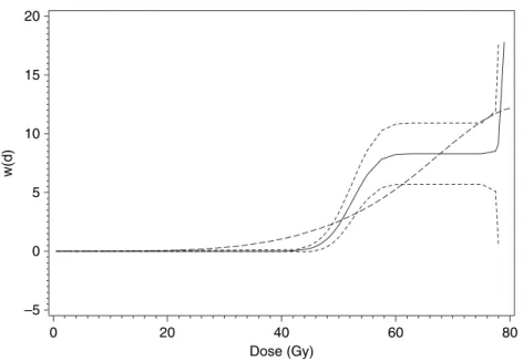
The maximum likelihood estimate and 95% pointwise confidence intervals ofw.d/are shown in Fig. 3. Very similar results are obtained with different choices forr.d/(two knots at 25 and 50 Gy or three knots at 20, 40 and 60 Gy) andh.z/(exp(z) orz2). The pointwise confidence intervals are calculated by using a delta method estimate of the standard error. To interpret the estimatedw.d/, it is helpful to note that regression coefficients have both subject-specific and population-average interpretations in Poisson–normal random-intercept models. In other words, the marginal means still have the same exponential form except that the intercept is changed (Breslow and Clayton, 1993). Consider two parotid glands, say gland A and gland B, which are of the same type (ipsilateral or contralateral) but differ only in the dose of radiation received. Assume that gland A receives a uniform dosedc and gland B receives no dose of
radiation. LetμA andμBbe the expected saliva flows for glands A and B respectively. Then, from equation (9), some calculations show that log.μA/−log.μB/= −w.dc/:Thusw.dc/could
be interpreted as the difference in expected saliva flow (on the log-scale) between a gland that received uniform dosedcand a gland that received no dose of radiation. Similarly, exp{−w.dc/}
can be interpreted as the ratioμA=μB.
15
10
5
0
–5 20
Dose (Gy)
w(d)
0 20 40 60 80
Fig. 3. Maximum likelihood estimate and pointwise 95% confidence intervals ofw.d/: , generalized monotone functional mixed model estimate; - - - , 95% confidence interval; – – – , estimate by using I-splines
Table 1. Parameter estimates and stan-dard errors for the saliva flow data
Parameter Estimate Standard error
α0 1.23 0.09
α1 0.72 0.02
Σ11 11.77 3.01
Σ12 0.005 0.17
Σ22 0.72 0.12
ratio test by testingH0:β1=β2=. . .=β6. Theχ2-statistic withp-value in parentheses for the likelihood ratio test is 29.9 (p <0:0001/. Thus we strongly reject the mean dose model in favour of our non-parametric model.
Estimates of the baseline saliva effect and the variance components are shown in Table 1. The results show that baseline saliva flow is a significant factor for saliva flow at month 6. Overdispersion for the ipsilateral and contralateral glands is captured byΣ1,1andΣ2,2 respec-tively. Overdispersion is significant for both but much larger for the ipsilateral glands. The correlation between glands could be measured by using the covariance parameter estimates Σ12=√.Σ11Σ22/=0:002, which is not significantly different from 0. A significantly negativeΣ12 would have given support to the notion of compensation whereas a significantly positive cor-relation would indicate that the two glands within a subject tend to behave similarly. We thus find no support for the notion of compensation between glands.
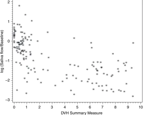
Fig. 4 plots, for each gland, the log-proportion change in saliva flow against the estimated summary measure of the dose effectΣk=164
k=2 pij.dk/wˆ.dk/. Because some of the saliva flows are
DVH Summary Measure
log (Saliv
a flo
w/Baseline)
0 2
1 2 3 4 5 6 7 8 9 10
1
0
–1
–2
–3
Fig. 4. Change in log-saliva-flow from baselineversusestimated dose effect summary measure
given by equation (9) since ˆα1=1. However, the plot changes very little if instead we plot log{.Yij+1/=.αˆ1baseij+1/}. There is clearly a decreasing and approximately linear trend. It
is also apparent that there is substantial variation in the change in saliva flows from baseline, even at a fixed dose effect level. Some of this variation is due to variability between glands and subjects.
The NTCP model is equivalent to a probit regression model with a power law mean dose term for the linear predictor:
NTCPij=Φ
β0+β1
164
k=2
dkλpij.dk/
1=λ
.11/
where NTCPijis the probability of complication for thejth gland of theith subject. This model cannot be directly compared with the generalized monotonic functional mixed model that we used to analyse the saliva data because it applies to binary outcomes. It is, however, possible to compare how each model summarizes the dose effect. To do so we replace the summary measure of dose effect in model (10) with the summary measure of dose effect in the NTCP model and fit the model with mean given by
log.μij/=α0+α1baseij+α2 164
k=2
dkλpij.dk/
1=λ
+bij: .12/
An alternative approach to estimatingw.d/monotonically is to approximatew.d/directly by using a regression spline withI-spline basis functions (Ramsay, 1988) asw.d/=ΣLl=+41βlIl.d/,
where theβls are constrained to be positive andIl.d/=
d
0 Bl.c/dcare theI-spline basis func-tions defined as the integral of theB-spline basis functions and are thus monotone increasing. We used this approach to estimatew.d/for the month 6 saliva flow data. Of the six param-eters, two were estimated to be at the boundary value of 0. The resulting estimate ofw.d/is shown in Fig. 3 and is somewhat different from the generalized monotonic functional mixed model estimate. Rather than being flat for doses up to 50 Gy, theI-spline estimator starts to increase after 30 Gy and is more linear thereafter than our estimate. We show in the simulation study in Section 5 thatI-splines do not work well for estimating flat regions. The associated −2 log-likelihoods are 1105.4, 1079.5 and 1075.5 for models that are based on the mean dose,
I-spline and our method respectively. TheI-spline model and our model have the same number of parameters and likelihood values favour our model, although we cannot test this, since the two models are not nested.
4.4. Goodness of fit
Goodness-of-fit statistics are used to assess whether the model fits the data reasonably well. One commonly used such statistic is the PearsonX2-statistic and is computed as
i
j
.yij−μij/2=μij .13/
whereμij=E[yij|bi] is the conditional mean and is obtained from equation (9) by plugging in
estimates of the fixed effect parametersαandβand of the random-effect estimatesbi.
Condi-tional on the random effectbi,Yijfollows a Poisson distribution and so the variance is simply
equal to the (conditional) mean and thus we divide byμij. There are two variants on statistic (13) that we also consider. The first is obtained with the same numerator but a different stan-dardization. Rather than dividing byμij, we divide by the conditional mean-squared error of prediction (Booth and Hobert, 1998). Doing so accounts for the variability in the estimates of the random effects. The second is to subtract the marginal mean and to divide by the marginal variance ofYij. For a detailed discussion of goodness of fit in generalized non-linear mixed
models, and in particular how residuals that are based on marginal and conditional means are sensitive to different model assumptions, see Voneshet al.(1996). The null distribution of these statistics is not known, so we use a parametric bootstrap approach to obtain empirical esti-mates. Specifically we simulate 100 data sets of the same size as our observed data set, using the parameter estimates from the observed data. For each data set we fit the model and compute the goodness-of-fit statistic. Of the 100 simulated data sets, 21 had goodness-of-fit statistics (based on the marginal mean and variance) that were larger than that of our observed data. Results are similar (p-values 0.55 and 0.15) for the other two goodness-of-fit statistics. Thus, on the basis of these metrics, our proposed model appears to be consistent with the data.
5. Simulations
log.μi/=α0−
k=164
k=2
w.dk/ pi.dk/ .14/
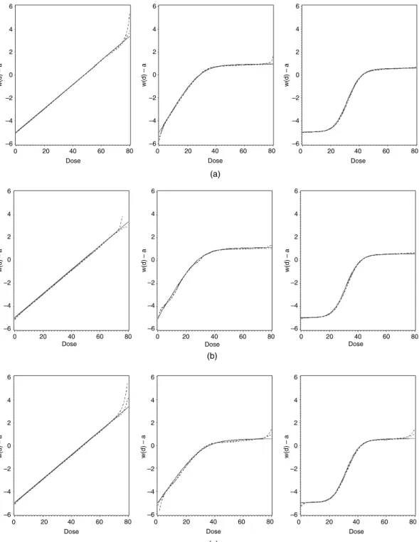
where we set α0=5, which is roughly the mean of the sum of the estimated intercept and baseline flow terms in the observed data. To mimic the saliva data, the DVHs were simulated as normal densities (truncated to lie in (0,82)) with means drawn uniformly in (5,76.5) and standard deviations drawn uniformly on (1,10). Fig. 5 shows the mean and median of the estimated values of w.d/−α0 for each shape along with the underlying true w.d/−α0. We have usedw.d/−α0because estimates of this quantity are more stable than estimates ofw.d/ alone.
We next conduct a simulation study to assess the performance of this method for overdispersed Poisson data such as the saliva flow data. We simulate data by using the model
log.μi/=α0−
k=164
k=2
w.dk/ pi.dk/+bi
where we setα0=5 and the random effectsbi∼N.0, 1/. We simulate 100 data sets of size 157 for
each of the three different shapes ofw.d/. The results are shown in Fig. 5. For both the Poisson and the overdispersed Poisson data, there is little bias except in the tails. There are relatively little data in these regions for some of the simulated data sets so the estimates tend to be more variable with a few extreme estimates having a large effect on the mean.
We wished to assess the robustness of our proposed estimator to the choice ofh.·/. To do so we analysed the Poisson data sets that were discussed above, which were generated by using h.z/=1000φ.z/, withh.z/=z2. The results are in Fig. 5, where we see no evidence of bias from using a differenth.·/function in the analysis. We also wished to assess the robustness of our proposed estimator to the choice of the number of knots that are used to definer.d/. To do so we generated 100 simulated data sets as discussed above by using a three-knot regression spline formulation forr.d/with knots at 20, 40 and 60 Gy. We then analysed these data sets by using a two-knot regression spline with knots at 30 and 55 Gy. The results (which are not shown) indicate a good fit with no evidence of bias.
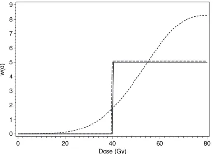
To illustrate the increased flexibility in our estimator compared with theI-spline estimator, we consider the extreme case wherew.d/is a step function. We simulate a single Poisson data set based on thisw.d/from equation (14). We then fit both our model and theI-spline-based model to these data. The resulting estimates are shown in Fig. 6. TheI-spline method severely oversmooths this step function. The reason for this is that the slope and maximum value of theI-regression spline are linked. To obtain a steeper function, we need a larger parameter coefficient, which also means a larger maximum value. It is thus not possible to obtain a ‘small steep’ increase. To be fair, our method is also not ideally suited to estimating step functions. Extremely large parameter values are required to do so. Our method also suffers from a lack of identifiability whenw.d/is a step function, because there are many sets of parameters that yield nearly identical estimates. This complicates tasks such as computing confidence intervals forw.d/. Nevertheless, the method can indicate whether the true function being estimated is a step function.
6. Discussion
6 4 2 –4 –2 –6 0 0
20 40 60 80 Dose
w(d) – a
6 4 2 –4 –2 –6 0 0
20 40 60 80 Dose
w(d) – a
6 4 2 –4 –2 –6 0
w(d) – a
0 20 40 60 80
Dose (a) (b) 6 4 2 –4 –2 –6 0 0
20 40 60 80 Dose
0 20 40 60 80 Dose
0 20 40 60 80 Dose
w(d) – a
6 4 2 –4 –2 –6 0
w(d) – a
6 4 2 –4 –2 –6 0
w(d) – a
6 4 2 –4 –2 –6 0
w(d) – a
6 4 2 –4 –2 –6 0
w(d) – a
6 4 2 –4 –2 –6 0
w(d) – a
(c)
0 20 40 60 80
Dose
0 20 40 60 80
Dose
0 20 40 60 80
Dose
Dose (Gy)
w(d)
8 9
7
6
4 5
3
2
1
0
0 20 40 60 80
Fig. 6. Comparison of our method and theI-spline method for estimating a step function: , true function; - - - ,I-spline estimator; – – – , our estimator
estimating a monotone weight functionw.d/, which includes several commonly used summaries such as the mean dose as special cases. This non-parametric method is in contrast with typical radiobiological models which tend to be highly parametric. Simulations for both Poisson and overdispersed Poisson data show that the method performs well in estimating various shapes of the weight functionw.d/.
There are two principal uses of the model that is presented in this paper. The first is to aid in the choice of treatment plan. To choose between multiple potential treatments plans for a new patient, the radiation oncologist could choose the plan with the lowest value of Σ164
k=1pij.dk/w.dk/. Alternatively the non-parametric estimate can be used to motivate a
para-metric summary measure. For instance the non-parapara-metric estimate ofw.d/in Fig. 3 is similar to a step function with a step at 50 Gy. Thus, rather than using ˆw.d/, the radiation oncologist could instead use V50, the proportion of the gland receiving a dose more than 50 Gy, which is easier to compute, to choose between plans. The second use of our proposed model is in pre-diction. Predicted saliva flow rates 6 months after treatment with a given plan can be obtained from equation (10) by plugging in parameter estimates. To obtain expected rates for an average patient, the random effectbijcould be replaced by 0.
In comparing our estimator with the estimator that is based onI-spline functions with the same number of knots, we found our method to be more flexible especially for flat regions. It also does not require constraints on the regression parametric space. We consider in this paper a regression spline method. A key advantage of the regression spline approach is that it is compu-tationally easy. Drawbacks include unstable behaviour near the end points as well as the need to choose the number and placement of knots. The data example and simulation study, however, show that the regression spline method works well in modelling our normal tissue complication data except for the boundary. An alternative approach is to use smoothing splines (Green and Silverman, 1994) andP-splines (Ruppertet al., 2003). A major disadvantage of such approaches is computational burden, especially for non-linear mixed models for non-Gaussian outcomes.
explicictly allows for flat regions is desirable. Dunson (2005) proposed such a method within a Bayesian framework, for relating a scalar dose value with a scalar outcome. This approach could be adapted to estimatew.d/within the generalized monotone functional mixed model that is proposed in this paper. The results are in Schipperet al.(2007).
References
Booth, J. G. and Hobert, J. P. (1998) Standard errors of prediction in generalized linear mixed models.J. Am. Statist. Ass.,93, 262–272.
Breslow, N. E. and Clayton, D. G. (1993) Approximate inference in generalized linear mixed models.J. Am. Statist. Ass.,88, 9–25.
Dunson, D. B. (2005) Bayesian semiparametric isotonic regression for count data.J. Am. Statist. Ass.,100, 618–627.
Eisbruch, A., TenHaken, R. K., Kim, H. M., Marsh, L. H. and Ship, O. (1999) Dose, volume, and function relationships in parotid salivary glands following conformal and intensity-modulated irradiation of head and neck cancer.Int. J. Radian. Oncol. Biol. Phys.,45, 577–587.
Friedman, J. and Tibshirani, R. (1984) The monotone smoothing of scatterplots.Technometrics,26, 243–250. Gelfand, A. E. and Kuo, L. (1991) Nonparametric Bayesian bioassay including ordered polytomous response.
Biometrika,78, 657–666.
Green, P. J. and Silverman, B. W. (1994)Nonparametric Regression and Generalized Linear Models. London: Chapman and Hall.
Hall, P. and Huang, L. (2001) Nonparametric kernel regression subject to monotonicity constraints.Ann. Statist., 29, 624–647.
Holmes, C. C. and Heard, N. A. (2003) Generalised monotonic regression using random change points.Statist. Med.,22, 623–638.
James, G. M. (2002) Generalized linear models with functional predictors.J. R. Statist. Soc.B,64, 411–432. Johnson, T. D., Taylor, J. M. G., TenHaken, R. K. and Eisbruch, A. (2005) A Bayesian mixture model relating
dose to critical organs and functional complication in 3D conformal radiation therapy.Biostatistics,6, 615–632. Kelly, C. and Rice, J. (1990) Monotone smoothing with application to dose-response curves and the assessment
of synergism.Biometrics,46, 1071–1085.
Kutcher, G. J., Burman, C. and Brewster, L. (1989) Calculation of complication probability factors from non-uniform tissue irradiation: the effective volume method.Int. J. Radian Oncol. Biol. Phys.,16, 1623–1630. Lichter, A. S. (1991) Three-dimensional conformal radiation therapy: a testable hypothesis.Int. J. Radian Oncol.
Biol. Phys.,21, 853–855.
Lyman, J. T. (1985) Complication probability as assessed from dose-volume-histograms.Radian Res.,104, 513– 519.
McCullagh, P. and Nelder, J. A. (1989)Generalized Linear Models, 2nd edn. London: Chapman and Hall. Pinheiro, J. C. and Bates, D. M. (1995) Approximations to the log-likelihood function in the non-linear
mixed-effects model.J. Computnl Graph. Statist.,4, 12–35.
Ramsay, J. O. (1988) Monotone regression splines in action.Statist. Sci.,3, 425–461.
Ramsay, J. O. (1998) Estimating smooth monotone functions.J. R. Statist. Soc.B,60, 365–375. Ramsay, J. O. and Silverman, B. W. (1997)Functional Data Analysis, pp. 157–177. New York. Springer. Ruppert, D., Wand, M. P. and Carroll, R. J. (2003)Semiparametric Regression. Cambridge: Cambridge University
Press.
Schipper, M. J., Taylor, J. M. G. and Lin, X. (2007) Bayesian generalized monotonic functional mixed models for the effects of radiation dose histograms on normal tissue complications.Statist. Med.,26, 4643–4656. Vonesh, E. F., Chinchilli, V. M. and Pu, K. (1996) Goodness-of-fit in generalized nonlinear mixed models.
Bio-metrics,52, 572–587.