R E S E A R C H
Open Access
A superlinearly convergent hybrid algorithm
for systems of nonlinear equations
Lian Zheng
**Correspondence: [email protected] Department of Mathematics and Computer Science, Yangtze Normal University, Fuling, Chongqing, 408100, China
Abstract
We propose a new algorithm for solving systems of nonlinear equations with convex constraints which combines elements of Newton, the proximal point, and the projection method. The convergence of the whole sequence is established under weaker conditions than the ones used in existing projection-type methods. We study the superlinear convergence rate of the new method if in addition a certain error bound condition holds. Preliminary numerical experiments show that our method is efficient.
MSC: 90C25; 90C30
Keywords: nonlinear equations; projection method; global convergence; superlinear convergence
1 Introduction
LetF:Rn→Rnbe a continuous mapping andC⊂Rnbe a nonempty, closed, and convex set. The inner product and norm are denoted by·,·and · , respectively. Consider the problem of finding
x*∈C such that Fx*= . (.)
Let S denote the solution set of (.). Throughout this paper, we assume thatS is nonempty andFhas the property that
F(y),y–x*≥, for ally∈Cand allx*∈S. (.) The property (.) holds ifFis monotone or more generally pseudomonotone onCin the sense of Karamardian [].
Nonlinear equations have wide applications in reality. For example, many problems aris-ing from chemical technology, economy, and communications can be transformed into nonlinear equations; see [–]. In recent years, many numerical methods for problem (.) with smooth mappingFhave been proposed. These methods include the Newton method, quasi-Newton method, Levenberg-Marquardt method, trust region method, and their variants; see [–].
Recently, the literature [] proposed a hybrid method for solving problem (.), which combines the Newton, proximal point, and projection methodologies. The method pos-sesses a very nice globally convergent property ifFis monotone and continuous. Under
the assumptions of differentiability and nonsingularity, locally superlinear convergence of the method is proved. However, the condition of nonsingularity is too strong. Relaxing the nonsingularity assumption, the literature [] proposed a modified version for the method by changing the projection way, and showed that under the local error bound condition which is weaker than nonsingularity, the proposed method converges superlinearly to the solution of problem (.). The numerical performances given in [] show that the method is really efficient. However, the literatures [, ] need the mappingFto be monotone, which seems too stringent a requirement for the purpose of ensuring global convergence property and locally superlinear convergence of the hybrid method.
To further relax the assumption of monotonicity ofF, in this paper, we propose a new hybrid algorithm for problem (.) which covers one in []. The global convergence of our method needs only to assume thatFsatisfies the property (.), which is much weaker than monotone or more generally pseudomonotone. We also discuss the superlinear con-vergence of our method under mild conditions. Preliminary numerical experiments show that our method is efficient.
2 Preliminaries and algorithms
For a nonempty, closed, and convex set⊂Rnand a vectorx∈Rn, the projection ofx ontois defined as
(x) =arg min
y–x|y∈.
We have the following property on the projection operator; see [].
Lemma . Let⊂Rnbe a closed convex set. Then it holds that
x–(y)
≤ x–y–y–(y)
, ∀x∈,y∈Rn.
Algorithm . Choosex∈C, parametersκ∈[, ),λ,β∈(, ),γ,γ> ,a,b≥,
max{a,b}> , and setk:= .
Step . ComputeF(xk). IfF(xk) = , stop. Otherwise, letμ
k=γF(xk)/,
σk=min{κ,γF(xk)/}. Choose a positive semidefinite matrixGk∈Rn×n.
Computedk∈Rnsuch that
Fxk+ (Gk+μkI)dk=rk, (.)
where
rk≤σkμkdk. (.)
Stop ifdk= . Otherwise,
Step . Computeyk=xk+t
kdk, wheretk=βmk andmkis the smallest nonnegative
integermsatisfying
–Fxk+βmdk,dk≥λ( –σk)μkdk
Step . Compute
xk+=Ck
xk–αkF
yk,
whereCk:={x∈C:hk(x)≤}and
hk(x) :=
aFxk+bFyk,x–yk+atk
Fxk,dk, (.) αk:=
F(yk),xk–yk
F(yk) .
Letk=k+ and return to Step .
Remark . When we take parametersa= ,b= , and the search directiondk=x¯k–
xk, our algorithm degrades into one in []. At this step of getting the next iterate, our projection way and projection region are also different from the one in [].
Now we analyze the feasibility of Algorithm .. It is obvious thatdksatisfying condi-tions (.) and (.) exists. In fact, when we takedk= –(G
k+μkI)–F(xk),dksatisfies (.) and (.). Next, we need only to show the feasibility of (.).
Lemma . For all nonnegative integer k, there exists a nonnegative integer mk
satisfy-ing (.).
Proof Ifdk= , then it follows from (.) and (.) thatF(xk) = , which means Algo-rithm . terminates withxkbeing a solution of problem (.).
Now, we assume thatdk= , for allk. By the definition ofrk, the Cauchy-Schwarz in-equality and the positive semidefiniteness ofGk, we have
–Fxk,dk=dkT(Gk+μkI)
dk–dkTrk
≥μkdk
–rkdk
≥( –σk)μkdk. (.)
Suppose that the conclusion of Lemma . does not hold. Then there exists a nonnegative integerk≥ such that (.) is not satisfied for any nonnegative integerm,i.e.,
–Fxk+βmdk,dk<λμ
k( –σk)d
k, ∀m. (.)
Lettingm→ ∞and by the continuity ofF, we have
–Fxk,dk≤λμ
k( –σk)d k.
Which, together with (.),dk= , andσ
3 Convergence analysis
In this section, we first prove two lemmas, and then analyze the global convergence of Algorithm ..
Lemma . If the sequences{xk}and{yk}are generated by Algorithm .,{xk}is bounded and F is continuous, then{yk}is also bounded.
Proof Combining inequality (.) with the Cauchy-Schwarz inequality, we obtain
μk( –σk)dk≤–
Fxk,dk
≤Fxkdk.
By the definition ofμkandσk, it follows that
dk≤ F(x k)
μk( –σk)≤
F(xk)/ γ( –κ) .
From the boundedness of{xk}and the continuity ofF, we conclude that{dk}is bounded, and hence so is{yk}. This completes the proof.
Lemma . Let x*be a solution of problem (.) and the function h
kbe defined by (.). If condition (.) holds, then
hk
xk≥λbtk( –σk)μkdk
and hk
x*≤. (.)
In particular, if dk= , then hk(xk) > .
Proof
hk
xk=aFxk+bFyk,xk–yk+atk
Fxk,dk =aFxk, –tkdk
+bFyk, –tkdk
+atk
Fxk,dk = –btk
Fyk,dk (.)
≥λbtk( –σk)μkdk
, (.)
where the inequality follows from (.).
hk
x*=aFxk+bFyk,x*–yk+atk
Fxk,dk
=aFxk,x*–xk+aFxk,xk–yk+bFyk,x*–yk+atk
Fxk,dk
≤,
where the inequality follows from condition (.) and the definition ofyk.
Ifdk= , thenhk(xk) > becauseσk≤κ< . The proof is completed.
Remark . Lemma . means that the hyperplane
Hk:=
x∈Rn|aFxk+bFyk,x–yk+atk
Fxk,dk=
Letx*∈Sanddk= . Since
aFxk+bFyk,xk–x*=aFxk,xk–x*+bFyk,xk–x*
=aFxk,xk–x*+bFyk,xk–yk+bFyk,yk–x*
≥bFyk,xk–yk
≥λbtkμk( –σk)dk
> ,
where the first inequality follows from condition (.), the second one follows from (.), and the last one followsdk= , which shows that –(aF(xk) +bF(yk)) is a descent direction of the function
x–x
*at the pointxk.
We next prove our main result. Certainly, if Algorithm . terminates at Stepk, thenxk is a solution of problem (.). Therefore, in the following analysis, we assume that Algo-rithm . always generates an infinite sequence.
Theorem . If F is continuous on C, condition (.) holds andsupkGk<∞, then the sequence{xk} ⊂Rngenerated by Algorithm . globally converges to a solution of (.).
Proof Letx*be a solution of problem (.). Sincexk+= Ck(x
k–α
kF(yk)), it follows from Lemma . that
xk+–x*≤xk–αkF
yk–x*–xk+–xk+αkF
yk =xk–x*– αk
Fyk,xk–x*–xk+–xk– αk
Fyk,xk+–xk,
i.e.,
xk–x*–xk+–x*≥αk
Fyk,xk–x*+xk+–xk+ αk
Fyk,xk+–xk
≥αk
Fyk,xk–yk+xk+–xk+αkF
yk–αkFyk
≥αk
Fyk,xk–yk–αkFyk =F(y
k),xk–yk
F(yk) ,
which shows that the sequence{xk+–x*}is nonincreasing, and hence is a convergent sequence. Therefore,{xk}is bounded and
lim
k→∞
F(yk),xk–yk
F(yk) = . (.)
From Lemma . and the continuity ofF, we have that{F(yk)}is bounded; that is, there exists a positive constantMsuch that
By (.) and the choices ofσkandλ, we have
F(yk),xk–yk F(yk) =
t
kF(yk),dk
F(yk)
≥tkλ( –σk)μkdk M
≥λ( –κ)tkμkdk
M .
This, together with inequality (.), we deduce that
lim
k→∞tkμk
dk= .
Now, we consider the following two possible cases: Suppose first thatlim supk→∞tk> . Then we must have
lim inf
k→∞ μk= or lim infk→∞
dk= .
From the definition ofμk, the choice ofdkandsupkGk<∞, each case of them follows that
lim inf
k→∞
Fxk= .
SinceFis continuous and{xk}is bounded, which implies that the sequence{xk}has some accumulation pointxˆsuch that
F(x) = .ˆ
This shows thatxˆis a solution of problem (.). Replacingx*byxˆin the preceding argu-ment, we obtain that the sequence{xk–xˆ}is nonincreasing, and hence converges. Since
ˆ
xis an accumulation point of{xk}, some subsequence of{xk–xˆ}converges to zero, which implies that the whole sequence{xk–xˆ}converges to zero, and hencelim
k→∞xk=x.ˆ
Suppose now thatlimk→∞tk= . Letx¯be any accumulation point of{xk}and{xkj}be the corresponding subsequence converging tox. By the choice of¯ tk, (.) implies that
–Fxkj+t
kjβ
–dkj,dkj<λ( –σ
kj)μkjd
kj, for allj.
SinceFis continuous, we obtain by lettingj→ ∞that
–Fxkj,dkj≤λ( –σ
kj)μkjd
kj. (.)
From (.) and (.), we conclude thatλ≥, which contradictsλ∈(, ). Hence, the case oflimk→∞tk= is not possible. This completes the proof.
4 Convergence rate
In this section, we provide a result on the convergence rate of the iterative sequence gen-erated by Algorithm .. To establish this result, we need the following conditions (.) and (.).
Forx*∈S, there are positive constantsδ,c
, andcsuch that
cdist(x,S)≤F(x), ∀x∈N
x*,δ, (.)
and
F(x) –F(y) –Gk(x–y)≤cx–y, ∀x,y∈N
x*,δ, (.)
wheredist(x,S) denotes the distance fromxto solution setS, and
Nx*,δ=x∈Rn|x–x*≤δ.
IfFis differentiable and∇F(·) is locally Lipschitz continuous with modulusθ> , then there exists a constantL> such that
F(y) –F(x) –∇F(x)(y–x)≤Ly–x, ∀x,y∈N
x*,δ. (.)
In fact, by the mean value theorem of vector valued function, we have
F(y) –F(x) –∇F(x)(y–x)
=
∇Fτy+ ( –τ)x(y–x)dτ–
∇F(x)(y–x)dτ
≤
∇Fτy+ ( –τ)x–∇F(x)y–xdτ
≤θy–x
τdτ
=Ly–x,
whereL=θ/. Under assumptions (.) or (.), it is readily shown that there exists a constantL> such that
F(y) –F(x)≤Ly–x, ∀x,y∈N
x*,δ. (.)
In , the literature [] showed that their proposed method converged superlinearly when the underlying functionFis monotone, differentiable with∇F(x*) being nonsingu-lar, and∇Fis locally Lipschitz continuous. It is known that the local error bound condition given in (.) is weaker than the nonsingular. Recently, under conditions (.), (.), and the underlying functionF being monotone and continuous, the literature [] obtained the locally superlinear rate of convergence of the proposed method.
Lemma . Let G∈Rn×nbe a positive semidefinite matrix andμ> . Then () (G+μI)– ≤
μ;
() (G+μI)–G ≤.
Proof See [].
Lemma . Suppose that F is continuous and satisfies conditions (.), (.), and (.). If there exists a positive constant N such thatGk ≤N for all k, then for all k sufficiently large,
() cdk ≤ F(xk) ≤cdk; () F(xk) +G
kdk ≤cdk/, wherec,candcare all positive constants.
Proof For (), letxk∈N(x*,
δ) andxˆk∈Sbe the closest solution toxk. We have
xˆk–x*≤xˆk–xk+xk–x*≤δ,
i.e.,xˆk∈N(x*,δ). Thus, by (.), (.), (.), and Lemma ., we have
dk≤(Gk+μkI)–F
xk+(Gk+μkI)–rk
≤(Gk+μkI)–
Fxˆk–Fxk–Gk
ˆ
xk–xk +(Gk+μkI)–Gk
ˆ
xk–xk+ μk
rk
≤ c μk
xˆk–xk+ xˆk–xk+σkdk.
Byxk–xˆk=dist(xk,S) andσ
k≤κ, it follows that
( –κ)dk≤
c μk
distxk,S+
distxk,S.
From (.) and the choice ofμk, it holds that
c μk
distxk,S≤c –
cF(xk) γF(xk)/
= c γc
Fxk/.
From the boundedness of{F(xk)}, there exists a positive constantMsuch that
Fxk/≤M.
Therefore,
dk≤cM+ γc cγ( –κ)
distxk,S
≤cM+ γc c
γ( –κ)
Fxk. (.)
We obtain that the left-hand side of () by settingc:= c
For the right-hand side part, it follows from (.) and (.) that
Fxk≤ Gk+μkIdk+rk
≤Gk+μkI+σkμkdk
≤(N+γM+κγM)dk.
We obtain the right-hand side part by settingc:=N+γM+κγM. For (), using (.) and (.), we have
Fxk+Gkdk≤μkdk+rk
≤( +σk)μkdk
≤( +κ)γF
xk/dk
≤( +κ)γc/ dk /
.
By settingc:= ( +κ)γc/ , we obtain the desired result.
Lemma . Suppose that the assumptions in Lemma . hold. Then for all k sufficiently large, it holds that
yk=xk+dk.
Proof Bylimk→∞xk=x*and the continuity ofF, we have
lim
k→∞F
xk=Fx*= .
By Lemma .(), we obtain that
lim
k→∞d
k= ,
which means thatxk+dk∈N(x*,δ) for allksufficiently large. Hence, it follows from (.) that
Fxk+dk=Fxk+Gkdk+Rk, (.) whereRk ≤cdk. Using (.) and (.), (.) can be written as
Fxk+dk= –μkdk+rk+Rk. (.) Hence,
–Fxk+dk,dk=μkdk,dk
–rkdk–Rkdk
≥μkdk
–σkμkdk
–cdk
=
– cd k
μk( –σk)
μk( –σk)dk
By Lemma .() and the choices ofμkandσk, forksufficiently large, we obtain
≥ – cd k
μk( –σk)
≥ – cc – F(xk) ( –κ)γF(xk)/
= –cc –
F(xk)/ ( –κ)γ ≥
λ,
where the last inequality follows fromlimk→∞F(xk) = .
Therefore,
–Fxk+dk,dk≥λμk( –σk)dk,
which implies that (.) holds withtk= for allksufficiently large,i.e.,yk=xk+dk. This
completes the proof.
From now on, we assume thatkis large enough so thatyk=xk+dk.
Lemma . Suppose that the assumptions in Lemma . hold. Setx˜k:=xk–α
kF(yk). Then for all k sufficiently large, there exists a positive constant csuch that
x˜k–yk≤cdk /
.
Proof Set
Hk=x∈Rn|Fyk,x–yk= .
Thenx˜k=H
k(x
k) andyk∈H
k. Hence, the vectorsxk–x˜kandyk–x˜kare orthogonal. That is,
yk–x˜k=yk–xksinθ
k=dksinθk, (.)
whereθkis the angle betweenx˜k–xkandyk–xk. Becausex˜k–xk= –αkF(yk) andyk–xk= dk, the angle betweenF(yk) and –μ
kdkis alsoθk. By (.), we obtain
Fyk––μkdk
=Rk+rk,
which implies that the vectors F(yk), –μ
kdk and Rk +rk constitute a triangle. Since
limk→∞μk=limk→∞γF(xk)/= andlimk→∞αk = . So for allksufficiently large, we have
sinθk≤ rk+Rk μkdk
≤σk+ cdk
≤γF
xk/+ cF(x k)
cγF(xk)/
=
γ+ c cγ
Fxk/,
which, together with (.) and Lemma .(), we obtain
yk–x˜k≤
γ+ c cγ
Fxk/dk
≤cdk/,
wherec=c/ (γ+ccγ). This completes the proof.
Now, we turn our attention to local rate of convergence analysis.
Theorem . Suppose that the assumptions in Lemma . hold. Then the sequence
{dist(xk,S)}Q-superlinearly converges to.
Proof By the definition ofx˜k, Lemma .() and (.), for sufficiently largek, we have
x˜k–x*≤xk–αkF
yk–x*
≤xk–x*+F(y
k),xk–yk
F(yk) F
yk
≤xk–x*+dk
≤xk–x*+c– F
xk =xk–x*+c– Fxk–Fx*
≤ +Lc– xk–x*,
which implies thatlimk→∞˜xk–x*= becauselimk→∞xk–x*= . Thus,x˜k∈N(x*,δ)
forksufficiently large, which, together with (.), Lemma ., Lemma ., and the defini-tion ofx˜k, we obtain
Fx˜k≤Fxk+Gk
˜
xk–xk+cx˜k–xk
≤Fxk+Gk
yk–xk+Gkx˜k–yk+cx˜k–xk
≤cdk/+Ncdk/+cαkF
yk
≤(c+Nc)dk/+cdk =c+Nc+cdk
/ dk/
≤c+Nc+cc–/ F
xk/dk/.
Because{F(xk)}is bounded, there exists a positive constantcsuch that
Fx˜k≤cdk /
On the other hand, from Lemma ., we know that
S⊆C∩Hk,
where S is the solution set of problem (.). Since xk+ = C∩Hk(x˜
k), it follows from
Lemma . that
xk+–x*≤x˜k–x*–xk+–x˜k, ∀x*∈S,
which implies that
xk+–x*≤x˜k–x*.
Therefore, together with inequalities (.), (.), and (.), we have
distxk+,S≤distx˜k,S≤ c
Fx˜k
≤c c
dk/≤c c
cM+ γc cγ( –κ)
/
dist/xk,S,
which implies that the order of superlinear convergence is at least .. This completes the
proof.
Remark . Compared with the proof of the locally superlinear convergence in literatures [, ], our conditions are weaker.
5 Numerical experiments
In this section, we present some numerical experiments results to show the efficiency of our method. The MATLAB codes are run on a notebook computer with CPU.GHZ under MATLAB Version .. Just as done in [], we takeGk=F(xk) and use the left divi-sion operation in MATLAB to solve the system of linear equations (.) at each iteration. We chooseb= ,λ= .,κ= ,β= ., andγ= . ‘Iter.’ denotes the number of itera-tion and ‘CPU’ denotes the CPU time in seconds. We chooseF(xk) ≤–as the stop criterion. The example is tested in [].
Example Let F(x) = ⎛ ⎜ ⎜ ⎜ ⎝ – ⎞ ⎟ ⎟ ⎟ ⎠ ⎛ ⎜ ⎜ ⎜ ⎝ x x x x ⎞ ⎟ ⎟ ⎟ ⎠+ ⎛ ⎜ ⎜ ⎜ ⎝ x x x x ⎞ ⎟ ⎟ ⎟ ⎠+ ⎛ ⎜ ⎜ ⎜ ⎝ – – ⎞ ⎟ ⎟ ⎟ ⎠
and the constraint setCbe taken as
C=
x∈R
i=
xi≤,xi≥,i= , , ,
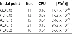
Table 1 Numerical results of Example witha= 10–15
Initial point Iter. CPU F(x*)
(3,0,0,0) 11 0.10 1.07×10⁻⁸
(1,1,0,0) 13 0.09 1.62×10⁻⁹
(0,1,0,1) 15 0.04 2.46×10⁻⁹
(0,0,0,1) 21 0.18 9.92×10⁻¹⁰
[image:13.595.226.369.200.267.2](1,0,0,2) 16 0.54 5.66×10⁻¹⁰
Table 2 Numerical results of Example witha= 0
Initial point Iter. CPU F(x*)
(3,0,0,0) 11 0.10 1.07×10⁻⁸
(1,1,0,0) 13 0.12 1.62×10⁻⁹
(0,1,0,1) 19 0.14 1.17×10⁻⁹
(0,0,0,1) 18 0.18 1.44×10⁻⁹
(1,0,0,2) 15 0.21 7.88×10⁻⁹
From Tables -, we can see that our algorithm is efficient if parameters are chosen prop-erly. We can also observe that the algorithm’s operation results change with the value ofa. When we takea= , the operation results are not best, that is to say, the directionF(yk) is not an optimal one.
Competing interests
The author declares that they have no competing interests.
Acknowledgements
The author wish to thank the anonymous referees for their suggestions and comments. This work is also supported by the Educational Science Foundation of Chongqing, Chongqing of China (Grant No. KJ111309).
Received: 28 March 2012 Accepted: 6 August 2012 Published: 24 August 2012 References
1. Karamardian, S: Complementarity problems over cones with monotone and pseudomonotone maps. J. Optim. Theory Appl.18, 445-454 (1976)
2. Dirkse, SP, Ferris, MC: MCPLIB: a collection of nonlinear mixed complementarity problems. Optim. Methods Softw.5, 319-345 (1995)
3. El-Hawary, ME: Optimal Power Flow: Solution Techniques, Requirement and Challenges. IEEE Service Center, Piscataway (1996)
4. Meintjes, K, Morgan, AP: A methodology for solving chemical equilibrium system. Appl. Math. Comput.22, 333-361 (1987)
5. Wood, AJ, Wollenberg, BF: Power Generations, Operations, and Control. Wiley, New York (1996) 6. Bertsekas, DP: Nonlinear Programming. Athena Scientific, Belmont (1995)
7. Dennis, JE, Schnabel, RB: Numerical Methods for Unconstrained Optimization and Nonlinear Equations. Prentice Hall, Englewood Cliffs (1983)
8. Ortega, JM, Rheinboldt, WC: Iterative Solution of Nonlinear Equations in Several Variables. Academic Press, San Diego (1970)
9. Polyak, BT: Introduction to Optimization. Optimization Software, Inc. Publications Division, New York (1987) 10. Tong, XJ, Qi, L: On the convergence of a trust-region method for solving constrained nonlinear equations with
degenerate solution. J. Optim. Theory Appl.123, 187-211 (2004)
11. Zhang, JL, Wang, Y: A new trust region method for nonlinear equations. Math. Methods Oper. Res.58, 283-298 (2003) 12. Fan, JY, Yuan, YX: On the quadratic convergence of the Levenberg-Marquardt method without nonsingularity
assumption. Computing74, 23-39 (2005)
13. Fan, JY: Convergence rate of the trust region method for nonlinear equations under local error bound condition. Comput. Optim. Appl.34, 215-227 (2006)
14. Fan, JY, Pan, JY: An improved trust region algorithm for nonlinear equations. Comput. Optim. Appl.48, 59-70 (2011) 15. Solodov, MV, Svaiter, BF: A globally convergent inexact Newton method for systems of monotone equations. In:
Fukushima, M, Qi, L (eds.) Reformulation: Piecewise Smooth, Semismooth and Smoothing Methods, pp. 355-369. Kluwer Academic, Dordrecht (1998)
16. Wang, CW, Wang, YJ: A superlinearly convergent projection method for constrained systems of nonlinear equations. J. Glob. Optim.44, 283-296 (2009)
17. Zarantonello, EH: Projections on Convex Sets in Hilbert Spaces and Spectral Theory. Academic Press, New York (1971) 18. Zhou, GL, Toh, KC: Superlinear convergence of a Newton-type algorithm for monotone equations. J. Optim. Theory
doi:10.1186/1029-242X-2012-180