Data Driven Three Phase Fundamental Diagram for Traffic Modeling

Data driven three-phase Fundamental Diagram for traffic

modeling

Jiah Song, [email protected]

Department of Mathematics, University of Michigan

Romesh Saigal, [email protected]

Department of Industrial and Operations Engineering, University of Michigan

Kang-Ching Chu, [email protected]

Department of Mechanical Engineering, University of Michigan

Qi Luo, [email protected]

Department of Industrial and Operations Engineering, University of Michigan

ABSTRACT

Macroscopic traffic flow models are widely used to estimate traffic status on a freeway, and the

fundamental diagram (FD), that establishes a relationship between density and flux, is essential for

these models to be effective. By visualizing the 2005 traffic trajectory data from Next Generation

SIMulation (NGSIM) project on US Highway 101 and Interstate 80 in California, we observed

three states of traffic condition: free flow, mildly congested flow, and highly congested flow; and

the resulting shockwaves. The FD is critical in understanding the shockwave phenomenon of

congested flow. Therefore, there is a need to develop a more accurate FD that captures the

complexity of the density-flux relation observed in the empirical data. For this we develop a three

phase FD of traffic flow.

In our previous work, a log piecewise linear FD was shown to fit better than some other

forms of FD on 2009 traffic data from Interstate 95 in Virginia. However, the previous FD

con-sidered two phases, free and congested flow. The three phase modification we propose here is

able to distinguish between the highly and the mildly congested flow and explains the resulting

shockwaves. The phase transition from mildly to highly congested state changes the nature of

the flux-density function from a concave to a convex function of density. In the concave phase

a forward moving and in the convex phase a backward moving shock results. This FD can also

explain the rarefaction waves that arise in traffic flow.

NGSIM data covers every vehicle within its range and we focus our study to the innermost

lane. The visualized data is used to fit the three phases. This involved solving an optimization

problem to determine the values of the parameters. A close relationship between the backward

shockwaves during highly congested phase and the convex part of the FD is observed. A single

parameter value (slope of the log-linear function) is shown to predict the various conditions of the

traffic: free, mildly and highly congested flow.

The proposed FD can be used in conjunction with any macroscopic traffic flow model, such

as LighthillWhithamRichards (LWR), for traffic flow estimation with greatly improved accuracy.

A three-phase FD and a stochastic macroscopic traffic flow model can reliably predict future

traffic status, and provide advanced information to drivers and transportation authorities for travel

1 INTRODUCTION

The performance of transportation system is crucial to economy and living quality of a community.

In 2014, traffic congestion in the US caused drivers 6.9 billion hours of extra time sitting in the

traffic and resulted in a congestion cost of $160 billion according to Schrank et al. (1). Managing

traffic and controlling congestion require an accurate estimation of traffic flow evolution. While

macroscopic traffic flow models and microscopic simulation tools are two main approaches for

traffic state estimation and prediction, because of their lower computational costs, macroscopic

models are favored for real-time application. Also macroscopic models can provide approximate

traffic status efficiently using scarce data collected from stationary detectors or trajectory data

from individual vehicles.

In macroscopic traffic flow, three variables, the flux (Q), the density (ρ) and the average

velocity/speed (v), where Q = ρv, are considered. The fundamental diagram (FD) is used to

model the relationship between density and flux. In addition, traffic flow is typically divided into

two states, free flow and congested flow, and it is particularly challenging to model congested flow

since the dynamics of congested traffic is more complex. Traffic shockwave phenomenon has been

clearly observed in the congested flow by Kerner (2), and a third phase called wide moving jam

is defined to distinguish it from typical congested traffic. For a macroscopic model to capture

this phenomenon, an explicit expression between flux and density (i.e. the FD) which sufficiently

explains the occurrence of traffic shock waves is required.

This paper presents a newly defined three-phase FD of traffic flow, where the objective is

to distinguish the formation and propagation of traffic shockwaves. The next section introduces

the required traffic theory background and an overview of the literature, followed by the proposed

model and theory. In the RESULTS section, two different sets of vehicle trajectory data from Next

Generation SIMulation, NGSIM (3), are used to validate proposed three-phase FD, as well as the

single parameter m. The last section states the conclusion of the presented work and proposes

future work and possible applications.

2 BACKGROUND AND RELATED WORK

The simple yet insightful LWR (Lighthill and Whitham (4), Richards (5)) model has been the

building block of macroscopic traffic flow models since its first appearance in 1955. The classical

LWR model, a nonlinear first order partial differential equation, treats traffic flow as a compressible

fluid and studies properties induced by the interaction of a group of vehicles. Although the LWR

model fails to explain several minor phenomena, such as hysteresis and traffic oscillations, indicated

by Li et al. (6), its hydrodynamic approach that implements mass conservation in traffic flow is

valid for homogeneous traffic flow. Many efforts have been made to improve LWR model, such as

including higher order term, adding source terms to flow conservation, and considering stochastic

nature of traffic. Some of the widely accepted higher order models include Payne (7), Aw and

Rascle (8), and Zhang (9). Yang et al. (10) proposed a stochastic partial differential equation

model building on the classic LWR traffic flow model to capture the variation of congestion and

gradual revert to the mean values after any random perturbations.

The LWR model allows discontinuous solutions in a weak sense and produces the

gener-ation and propaggener-ation of traffic shock waves. The speed of the shock wave, denoted by s, for a

jump fromρL toρR is

s= Q(ρR)−Q(ρL)

ρR−ρL

(1)

by the Rankine-Hugoniot condition, LeVeque (11). Here ρR represents the density to the right

of the shock, and ρL to the left of the shock. The shock speeds in (1) can be either positive or

negative, and this results in either forward-moving shock or backward-moving shock. It has been

relevant weak solution among multiple weak solutions. The details regarding entropy-satisfying

shock with our proposed flux-density relation will be described in the next section.

Besides traffic theories based on physics, sensor technology and the development of

intel-ligent transportation system allow researchers to use traffic data from real traffic and computer

simulations to better understand traffic phenomenon. Based on a thorough analysis using

empiri-cal data from German freeways, Kerner (2) proposed the three-phase traffic theory. Rather than

a single congestion state, congested traffic is divided into two phases, synchronized flow and wide

moving jam. According to Kerner’s definition, synchronized flow is when vehicles are continuously

moving under high density traffic, with possibly no significant drop in flux. On the other hand,

wide moving jam is caused by sudden drop in velocity with very high traffic density, and the jam

moves backwards across the space.

In macroscopic traffic models, vehicles can maintain constant velocity when density is low

(free flow), so the flux increases with density. In traffic with higher density the velocity decreases

and the flux may also decrease. The fundamental diagram (FD) captures this phenomenon with

the flux-density relationship. Other than the basic triangular FD, several forms of the FD have

been proposed in the past, and some of these have been frequently used in the literature. For

example, Greenshields et al. (12) considered a linear speed-density relationship as vf(1−ρ/ρj)

with free-flow velocityvf and critical density ρj as parameters. Also, Greenberg (13) proposed a

logarithmic relationship asv0ln(ρj/ρ) and Underwood (14) used exponential form,vfexp(−ρ/ρj).

Since some FDs are more appropriate for congested traffic while others are more suitable for free

flow, it is possible to mix them in application by adopting one in congested sections and another in

the free-flow sections. Yang et al. (10) proposed the log piecewise linear function to express

speed-density relation, which has been tested and shown to have the best fit among models mentioned

above in both free flow and congested flow regimes. Lu et al. (15) investigated a lane-wise FD

and proposed variable structure models with two limbs of the inverse λ−shape and a special

unique flux-density relationship in Kerner’s three-phase traffic theory, Treiber et al. (16) showed

that macroscopic traffic model with FD is capable of representing three-phase traffic. Daganzo

and Geroliminis (17) also pointed out that FD is not expected universally due to several factors

that dramatically affects the performance of congested flow in traffic.

Even for the stochastic traffic flow model with log piecewise linear FD used by Yang et al.

(10) and Chu et al. (18), the two-phase FD did not successfully reflect the complexity of traffic

congestion including traffic shock waves. This deficiency of the FD motivated us to modify the

log piecewise linear FD using the concept of three-phase traffic flow similar to Kerner’s theory,

and this allows phase transitions to be clearly defined by the range of a single exponent value in

fundamental relation formula.

3 MODEL AND THEORY

Throughout this paper, the following notation is used:

• (x, t) is the space and time, respectively.

• Q(x, t) is the flux, number of vehicles per unit time at location x and time t.

• ρ(x, t) is the density, number of vehicles per unit distance at location x and time t.

• v(x, t) is the average velocity of all vehicles at location x and time t.

In the rest of this paper, the independent variables (x,t) are omitted from the notation.

3.1 Three-Phase Fundamental Diagram

The LWR model consists of the scalar conservation law of mass (2) and the relationship among

Q, ρ andv, known as the fundamental relation of traffic flow (3),

∂ρ ∂t +

∂Q

Q = ρ·v. (3)

On a freeway, the vehicles tend to drive at some optimal velocity. That is to say, they drive at high

speed in light traffic and they slow down in heavy traffic. Therefore the velocity is dependent on

the local density. This additional information leads to the definition ofQ, which is a well-defined

function of the conserved quantity ρ. The fundamental diagram (FD) of traffic flow describes this

relationship betweenQandρ. It plays an important role in the use of the LWR model. Therefore,

to have a good predictive model, the FD should reflect the ’true’ relationship as accurately as

possible.

In our previous work, a log piecewise linear FD (4) was shown to fit better than some

other forms of FD on 2009 traffic data from Interstate 95 in Virginia, Yang et al. (10). This model

takes the form of

v= min{vf, αρm} (4)

where vf refers to the free flow velocity,m <0 andαis a constant. However, this original model

considered two phases, free and congested flow. In order to distinguish between the highly and

the mildly congested flow, we develop a modified log piecewise linear model that includes three

different phases. Themodified model is

v= min{vf, α∗ρm

∗

, αρ¯ m¯} (5)

where ¯m <−1< m∗ <0,α∗ and ¯αare constants, and vf refers to the free flow velocity. This

is called a modified log piecewiselinear model because (5) takes a piecewise linear form (see (7))

in a logarithm manner. It has been observed thatmis negative in the original model, Yang et al.

(10), and we divide thisminto two parameters,m∗ and ¯m, by a critical value−1 in the modified

value -1 came from the observation of backward-moving shockwave in traffic flow and

∂ρ

∂t +α(m+ 1)ρ m∂ρ

∂x = 0 (6)

obtained by manipulating (2) and (3). In (6), note that the information propagates to the left

whenm <−1, which results in the backward-moving shockwaves.

Now we describe our three-phase traffic flow in detail from the observation by

visualiz-ing the data, motivated by and similar to Kerner’s three-phase traffic theory but with different

definitions.

• The first or the free-flow phase (m = 0): This is when v is near the speed limit. In this

phase, we observe thatv is not affected byρ.

• The second or the mildly congested phase (−1 < m∗ < 0): We observed the presence of

data showing that traffic congestion begins to occur, that is,v decreases asρincreases. In

particular, this data shows the slow-down behavior is not as abrupt as in traffic jam. Note

that in a logarithm form, (5) takes

lnv= min{lnvf, lnα∗+m∗lnρ, ln ¯α+ ¯mlnρ}, (7)

so the negative slope in the (log) phase plane, lnvvs lnρ, is in between 0 and 1 in magnitude.

This is how−1< m∗<0 was derived in this second phase. Moreover, in this mildly congested

flow,Qstill increases as a concave function ofρ. We also claim that this phase is where the

forward-going shock may occur. This will be discussed in the next subsection.

• The third or the highly congested phase ( ¯m < −1): As ρ increases more and more, we

observed that v decreases quite abruptly. This results in the slope (in lnv and lnρ plane,

see (7)) being less than−1. Quantitatively this is where ¯m <−1 came from. This sudden

Density (vehicles/mile)

Flux (vehicles/hour)

Figure 1: The three-phase fundamental diagram. The dashed line is related to a forward-moving shock and the dash-dot line is related to a backward-moving shock.

WhileQincreases in the mildly congested phase,Qin this highly congested phase decreases

as a convex function ofρ.

FIGURE 1 illustrates the proposed three-phase FD; Qis an increasing linear function of

ρin the first phase (black). Qis an increasing and concave function ofρin the second phase (red)

while Q is a decreasing and convex function of ρ in the third phase (blue). We note that this

three-phase FD is not concave unlike the majority of proposed FD in the literature is concave.

3.2 Entropy Satisfying/Violating Shocks and Compound Waves

It is well known that the weak solutions of (2) are not in general unique, so the physically relevant

solution should be selected somehow and one way is to check the entropy condition. For more

details of non-uniqueness of weak solutions, we refer the reader to LeVeque (11). Furthermore,

due to the fact that the three-phase FD has a shape of non-convexity, we should expect to have

Riemann solutions with possibly both a shock and rarefaction fan. So in this subsection, we discuss

entropy-satisfying/violating shocks and compound waves. Note that the shock speedsin (1) can

be either positive or negative, which results in eitherforward-movingorbackward-moving shock.

• Forward-moving shock: In mildly congested flow, a vehicle slows down due to the behavior of

its preceding vehicle, and this effect continues to the following vehicle. Hence, the disturbance

why drivers do not notice the forward-going shock wave) while a rise in ρ may propagate

forward in space. Within the three-phase FD, several possibilities of forward-moving shock

may be considered whenρL< ρR. First, ifρLin the first phase jumps intoρR in the second

phase, then the Oleinik entropy condition is satisfied:

Q(ρL)−Q(ρ) ρL−ρ

≥ Q(ρL)−Q(ρR) ρL−ρR

(8)

for allρbetweenρL andρR. The dashed line in FIGURE 1 illustrates such forward-moving

shock. Second, if ρL in the second phase jumps into ρR in the second phase, then (8) is

also satisfied. Third, if ρL in the first phase jumps intoρR in the third phase, then (8) is

satisfied only whenQ(ρL)< Q(ρR). Lastly, if ρL in the second phase jumps intoρR in the

third phase, then (8) is also satisfied only in a very limited case whenQ(ρL)< Q(ρR). Phase

transition inρ may or may not be necessary for the forward-moving shock to be realized,

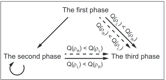
which is summarized in solid lines in FIGURE 2.

• Backward-moving shock : While the forward-moving shock is hardly observed in reality,

backward-moving shocks are easily observed. Within the three-phase FD, whenρR is in the

third phase and ρL is in the first phase as in the dash-dot line in FIGURE 1, the shock

propagates backwards in space due to the negative speed of the shocksin (1) (case 1). For

example, in a situation where the traffic is going fast, when the lead vehicle suddenly slows

down for some reason, ρ of following vehicles increases with a sudden slowdown. So there

is a jump in the value of ρ and this jump travels backwards in space. This single jump

could be represented as in the dash-dot line in FIGURE 1. In addition to that,ρR is in the

third phase and ρL in the second phase as in the red heavy line in FIGURE 3, the shock

also propagates backwards in space (case 2). In both cases, the entropy-satisfying shock

propagates backwards in space, provided that Q(ρR) < Q(ρL) under the Oleinik entropy

The first phase

The second phase

The third phase

Q( ρ

L) < Q(

ρ R) Q(

ρ

R) < Q(

ρ L)

Q(ρ_L) < Q(ρ_R)

Q(ρ_R) < Q(ρ_L)

Figure 2: Phase transitions when shock in density is generated. Solid lines imply the forward-moving shock while dashed lines imply the backward-forward-moving shock.

• Entropy-violating shock : With the three-phase FD, an entropy-violating shock wave can

arise. When both ρL and ρR are in the third phase and ρL < ρR, it is expected that a

backward-propagating shock wave is created. However, this violates the Entropy condition

as we can see from (8). This prediction of the three-phase FD needs explanation and is to

be investigated and researched further.

• Compound waves: When considering a non-convex flux function, it is known that the

Rie-mann solution might involve both a shock and a rarefaction wave. We present an example of

this. Taking the case ofρL in the third phase andρR in the second phase like the situation

along the red dotted line in FIGURE 3, the Riemann solution will contain both a rarefaction

and a shock propagating backwards. This illustrates thatρsuddenly drops fromρLto some

value of density through a shock wave and then toρRthrough a rarefaction.

4 DATA FITTING AND OPTIMIZATION OF PARAMETER m

The traffic dataset used in this paper to fit and validate the three-phase fundamental diagram

(FD) was collected under the Next Generation SIMulation (NGSIM (3)) project. Datasets from

the inner-most lane of US Highway 101 (US 101) and the lane 2 of Interstate 80 (I-80) were

used. US 101 data records vehicle trajectories and instantaneous velocity on the southbound of

Time (sec)

340 360 380 400 420 440 460

Space (ft)

500 1000 1500 2000

Vehicle trajectories

Figure 3: Vehicle trajectories of the NGSIM (US 101) around 7:55 a.m. to 7:57 a.m. on June 15th, 2005, along with backward-moving shock area (red line) and rarefaction wave area (red dotted line).

area is approximately 2,100 feet in length. The I-80 data of vehicle trajectories was recorded on

northbound direction of Interstate 80 in San Francisco, CA, between 4:00 p.m. and 4:15 p.m. on

April 13, 2005. The site is approximately 1,650 feet in length. Both (US 101 and I-80) vehicle

trajectory data provided the precise location of each vehicle within the study area every one-tenth

of a second with detailed lane positions. The following subsections contain two types of results:

the FD generated from the fitting of the speed-density relationship (i.e. the modified log piecewise

linear function) and the result of optimized parameterm.

4.1 Data fitting of Three-Phase Fundamental Diagram

In this subsection, we present the result of fitting of (7), which is the modified log piecewise linear

model. First, average velocity was calculated by the mean of recorded velocity data every 18

seconds and 50 feet and the FIGURE 4 (a) shows the average velocity of trajectory data of US

101. Flux was calculated by counting the number of vehicles in every 18 seconds. Then density

was computed by (3).

The fitting result of the speed-density relation in logarithm form and the corresponding

FD are presented in FIGURE 5. The FD is not universally expected according to Daganzo and

Geroliminis (17), and consequently it changes as region changes. In this context, two different

Time (sec)

0 200 400 600 800

Space (ft) 0 500 1000 1500 2000

Average velocity (mph)

10 20 30 40 50 60 70 Time (sec)

0 200 400 600 800

Space (ft) 0 500 1000 1500 2000

Map of optimized m a) b)

A

B

Figure 4: (a) Average velocity of 15 minutes (7:50 a.m. to 8:05 a.m.) of US 101 on June 15th, 2005. (b) Optimizedm.

piecewise linear function in a log form. Piecewise linear regression was applied to fit the data (after

taking the logarithm) in each of two regions A and B and to estimate each parameter (α, m).

By doing this, the data in each regions were segregated into two sections by a critical density, ρc,

which is determined by minimizing the sum of squares of the differences between observed and

computed ln(speed). The critical densities were turned out to be ρ∗_c = 24.7543 in region A as in

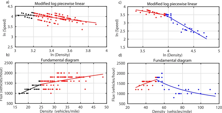
FIGURE 5 (b) and ¯ρc= 51.5731 in region B as in FIGURE 5 (d). The fitted results for the first

and the second phases in region A are as follows:

lnv = 4.0618 and (9)

lnv = −0.5588·lnρ+ 5.857, (10)

where (9) is shown as a black linear line and (10) is a red linear line in FIGURE 5 (a). FIGURE 5

three-ln (Density)

3 3.2 3.4 3.6 3.8 4

ln (Speed)

2.5 3 3.5 4

4.5 Modified log piecewise linear

Density (vehicles/mile)

15 20 25 30 35 40 45 50

Flux (vehicles/hour)

500 1000 1500 2000

2500 Fundamental diagram

a)

b) 3.5 ln (Density)4 4.5 5

ln (Speed) 1.5 2 2.5 3 3.5

4 Modified log piecewise linear

Density (vehicles/mile)

20 40 60 80 100 120

Flux (vehicles/hour)

500 1000 1500 2000

2500 Fundamental diagram

c)

d)

Figure 5: (a) The first and second phases of the three-phase flow on the modified log piecewise linear function in the region A of US 101 data. (b) The first and second phases of the three-phase flow on the fundamental diagram of traffic flow in the region A of US 101 data. (c) The second and third phases of the three-phase flow on the modified log piecewise linear function in the region B of US 101 data. (d) The second and third phases of the three-phase flow on the fundamental diagram of traffic flow in the region B of US 101 data.

phase flow as we expected from FIGURE 1. The fitted results for the second and third phases in

region B are as follows:

lnv = −0.542·lnρ+ 5.63 and (11)

lnv = −1.823·lnρ+ 10.68, (12)

where (11) is shown as a red linear line and (12) is a blue linear line in FIGURE 5 (c). FIGURE 5

(d) demonstrates the corresponding FD that provides the second and the third phases of the

three-phase flow as we also expected from FIGURE 1. As we observed backward-moving shocks in region

B from FIGURE 4 (a), the fitted result in FIGURE 5 (d) provides ¯m <−1 that is relevant to

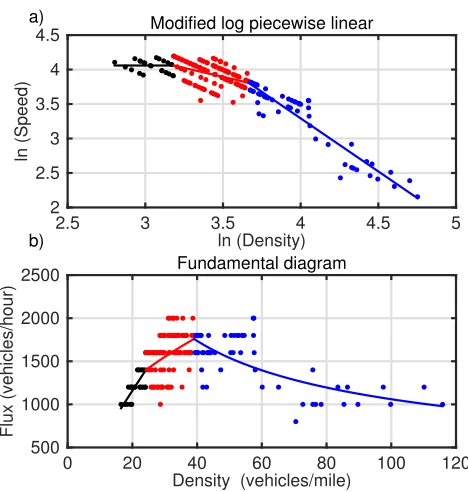
negative speed of shock. Moreover, putting data in region A and B together, we obtained the

ln (Density)

2.5 3 3.5 4 4.5 5

ln (Speed)

2 2.5 3 3.5 4

4.5 Modified log piecewise linear

Density (vehicles/mile)

0 20 40 60 80 100 120

Flux (vehicles/hour)

500 1000 1500 2000

2500 Fundamental diagram

a)

b)

Figure 6: (a) The three phases of the modified log piecewise linear function in the combined region A and B of US 101 data. (b) The three-phase fundamental diagram of traffic flow in the combined region A and B of US 101 data.

Table 1: Regression result of modified log piecewise linear model of US 101 data

Region Phase m lnα R2

A 2 -0.5588 5.857 0.2689

B 2 -0.542 5.63 0.4191

3 -1.823 10.68 0.8558

A and B combined 2 -0.5486 5.814 0.1978 3 -1.536 9.436 0.8901

of the modified log piecewise linear function in region A, region B, and the combined region. For

the fitting of combined region, the low R2 _{in the second phase is due to the mixed data from two}

different regions. The critical densities turned out to be 24.1190 (vehicles/mile) which separates

the first phase from the second phase and 39.0561 (vehicles/mile) which separates the second phase

from the third phase.

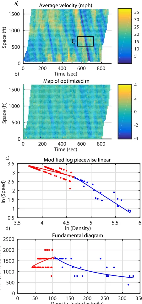
trajectory data of I-80 is presented in FIGURE 8 (a). This average velocity was calculated by the

mean of recorded velocity data every 9 seconds and 25 feet. The result of fiiting of the speed-density

function and the FD are presented in FIGURE 8 (c) and (d) with the second and third phases.

The first phase was not included because the average velocity ranges from 0 to approximately 37

mph as seen in FIGURE 8 (a). Fitted results of the modified piecewise linear function for I-80

dataset in region C illustrated in FIGURE 8 (a) are shown in Table 2 and FIGURE 8 (c). The

critical density turned out to be 105.2144 (vehicles/mile) in region C.

4.2 Optimization of parameter m

In this subsection, we attempt to optimizemover the entire space-time domain in order to identify

the role of parameter m. To find the optimized m for US 101 data, the space-time plane was

discretized by choosing a mesh width ∆x= 50 (feet) and a time step ∆t= 18 (sec), and defined the

discrete mesh points (xi, tj) byxi=i∆xandtj =j∆t. The parametermwas optimized based on

the assumption that change in density in the future on a highway depends on the past (backward

in time) information and the surrounding environment of drivers (centered in space). Namely,

m(xi, tj) is dependent upon v(xi+k, tj+l) and ρ(xi+k, tj+l) for k = −1,0,1, and l = −2,−1,0

where m(xi, tj) indicates numerical value of m at the discrete grid point (xi, tj). And then we

found

arg min

m,αklnv−mlnρ−lnαk 2 2.

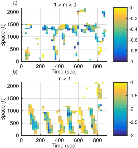
The result of the optimizedm of US 101 data is shown in FIGURE 4 (b). We can interpret that

mbeing−1 is a threshold that distinguishes the third phase from the second phase. On one hand,

the region where m = ¯m < −1 appears to be the third phase, and clearly there exists a shock

traveling backwards in space. On the other hand, in the region where −1< m=m∗ <0, there

appears to be the second phase. FIGURE 7 (a) depicts the region at where −1< m =m∗ <0

Time (sec)

0 200 400 600 800

Space (ft) 0 500 1000 1500 2000

-1 < m < 0

-1 -0.8 -0.6 -0.4 -0.2 0 Time (sec)

0 200 400 600 800

Space (ft) 0 500 1000 1500 2000 m <-1 a) b) -3 -2.5 -2 -1.5 -1

Figure 7: (a) Optimizedm only when−1< m <0 for US 101 data. (b) Optimizedm only when

m <−1 for US 101 data.

Table 2: Regression result of modified log piecewise linear model of I-80 data

Region Phase m lnα R2

C 2 -0.6699 5.889 0.4795 3 -1.742 10.88 0.8655

comparing the map of optimized m(in FIGURE 4 (b)) with the average velocity (in FIGURE 4

(a)). The result of the optimizedmof I-80 data is also shown in FIGURE 8 (b) (we used ∆x= 25

(feet) and ∆t = 9 (sec)). As we can see from those results, the value of m gives an indication

of how congested the traffic is. Again, the fact that the optimized m in FIGURE 8 (b) and the

average velocity in FIGURE 8 (a) match up well enough provides us a visual validation.

5 CONCLUSION

This paper presents a new approach to the three-phase fundamental diagram (FD) in macroscopic

Time (sec)

0 200 400 600 800

Space (ft) 0 500 1000 1500

Average velocity (mph)

5 10 15 20 25 30 35 Time (sec)

0 200 400 600 800

Space (ft) 0 500 1000 1500

Map of optimized m a) b)

C

3.5 4 4.5 5 5.5 6

ln (Speed) 0.5 1 1.5 2 2.5 3

3.5 Modified log piecewise linear

Density (vehicles/mile)

0 50 100 150 200 250 300 350

Flux (vehicles/hour) 0 500 1000 1500 2000

2500 Fundamental diagram

c)

d)

Figure 8: (a) Average velocity of 15 minutes (4:00 p.m. to 4:15 p.m.) of I-80 on June 15th, 2005. (b) Optimized m. (c) The second and third phases of the three-phase flow on the modified log piecewise linear function in the region C of I-80 data. (d) The second and third phases of the three-phase flow on the fundamental diagram of traffic flow in the region C of I-80 data.

(NGSIM) project on US Highway 101 and Interstate 80 in California. The result shows that the

congested flow), and it clearly shows the change in concavity in the FD. Furthermore, the single

parameterm, slope of the log-linear function, plays a crucial role as an indication to differentiate

the second phase from the third phase, and the critical mturns out to be−1.

The reason that the fit in the second phase is relatively poor compared to the fit in the

third phase could be the high variabilities in the second phase, which is not well captured by

the model we proposed. In our future work, we will use the LWR model or other appropriate

macroscopic traffic flow models along with the three-phase FD or possibly introduce stochasticity

to capture randomness of data and driver behavior to reliably predict future traffic status.

REFERENCES

[1] Schrank, D., B. Eisele, T. Lomax, and J. Bak, Urban mobility scorecard. Technical Report

August, Texas A&M Transportation Institute and INRIX, Inc, 2015.

[2] Kerner, B. S., Three-phase traffic theory and highway capacity. Physica A: Statistical

Me-chanics and its Applications, Vol. 333, 2004, pp. 379–440.

[3] NGSIM,Next Generation Simulation http://ngsim-community.org/, US Department of

Trans-portation, 2005.

[4] Lighthill, M. J. and G. B. Whitham, On kinematic waves. II. A theory of traffic flow on long

crowded roads. InProceedings of the Royal Society of London A: Mathematical, Physical and

Engineering Sciences, The Royal Society, 1955, Vol. 229, pp. 317–345.

[5] Richards, P. I., Shock Waves on the Highway.Operations Research, Vol. 4, No. 1, 1956, pp.

42–51.

[6] Li, J., Q.-Y. Chen, H. Wang, and D. Ni, Analysis of LWR model with fundamental diagram

[7] Payne, H. J., Models of freeway traffic and control.Mathematical models of public systems,

1971.

[8] Aw, A. and M. Rascle, Resurrection of ”second order” models of traffic flow. SIAM journal

on applied mathematics, Vol. 60, No. 3, 2000, pp. 916–938.

[9] Zhang, H. M., A non-equilibrium traffic model devoid of gas-like behavior. Transportation

Research Part B: Methodological, Vol. 36, No. 3, 2002, pp. 275–290.

[10] Yang, L., R. Saigal, C.-P. Chu, and Y.-W. Wan, Stochastic model for traffic flow prediction

and its validation. InTransportation Research Board 90th Annual Meeting, 2011, 11-0086.

[11] LeVeque, R. J., Numerical methods for conservation laws, Vol. 132. Springer, 1992.

[12] Greenshields, B., J. Bibbins, W. Channing, and H. Miller, A study of traffic capacity. In

Highway Research Board Proceedings, 1935.

[13] Greenberg, H., An analysis of traffic flow.Operations Research, Vol. 7, No. 1, 1959, pp. 79–85.

[14] Underwood, R., Speed, volume, and density relationships: Quality and theory of traffic flow.

Yale Bureau of Highway Traffic, New Haven, CT, 1961, pp. 141–188.

[15] Lu, X.-Y., P. Varaiya, and R. Horowitz, Fundamental Diagram modeling and analysis based

NGSIM data. In12th IFAC Symposium on Control in Transportation System, 2009, pp. 367–

374.

[16] Treiber, M., A. Kesting, and D. Helbing, Three-phase traffic theory and two-phase models

with a fundamental diagram in the light of empirical stylized facts. Transportation Research

Part B: Methodological, Vol. 44, No. 8-9, 2010, pp. 983–1000.

[17] Daganzo, C. F. and N. Geroliminis, An analytical approximation for the macroscopic

fun-damental diagram of urban traffic.Transportation Research Part B: Methodological, Vol. 42,

[18] Chu, K.-C., L. Yang, R. Saigal, and K. Saitou, Validation of stochastic traffic flow model

with microscopic traffic simulation. In 2011 IEEE Conference on Automation Science and