Quantifying alignment effects in 3D coordinate measurement

UMTRI-2009-40

OCTOBER

2009

Q

UANTIFYING

A

LIGNMENT

E

FFECTS IN

3D

C

OORDINATE

M

EASUREMENT

P

ATRICK

D.

H

AMMETT

,

P

H

D

L

UIS

M.

G

ARCIA

-G

UZMAN

S

TEVEN

W.

G

EDDES

QUANTIFYING ALIGNMENT EFFECTS

IN 3D COORDINATE MEASUREMENT

October 2009

Patrick C. Hammett, Ph.D.1 Luis M. Garcia-Guzman1

Steven W. Geddes1 Patrick T. Walsh2

Technical Report Documentation Page

1. Report No.

UMTRI-2009

2. Government Accession No. 3. Recipient’s Catalog No.

5. Report Date:

October 2009

4. Title and Subtitle

Quantifying Alignment Effects in 3D Coordinate Measurement

6. Performing Organization Code

7. Author(s)

Hammett, Patrick C., Garcia-Guzman, Luis M., Geddes, Steven W., and Walsh, Patrick T.

8. Performing Organization Report No.

UMTRI-2009

10. Work Unit no. (TRAIS) 9. Performing Organization Name and Address

The University of Michigan Transportation Research Institute 2901 Baxter Road

Ann Arbor, Michigan 48109-2150 U.S.A.

11. Contract or Grant No.

13. Type of Report and Period Covered 12. Sponsoring Agency Name and Address

14. Sponsoring Agency Code

15. Supplementary Notes

16. Abstract

The use of fixtureless, non-contact coordinate measurement has become increasingly prevalent in manufacturing problem solving. Manufacturers now routinely use measurement systems such as white light area scanners, photogrammetry, laser trackers, and portable laser scanners to conduct studies that require measuring upstream supplier parts, tooling, or in-process subassemblies. For part measurements in these studies, certified fixtures with alignment features such as tooling balls often are not available. Instead, manufacturers rely on ad hoc part-holding fixtures or measure parts without fixtures and perform alignments mathematically. Here, advancements in software are providing operators with numerous alignment options, and users are actively using this functionality. Naturally, these additional capabilities have led to inconsistencies in the alignment method used across measurement studies, often affecting dimensional results.

This paper reviews several common alignment or registration methods and provides a metric to assess systematic alignment error. To demonstrate alignment effects, we present a measurement system study of a moderately complex part requiring an over-constrained datum scheme. We first measure the part using a conventional fixture-based method to establish a baseline for static and dynamic repeatability. We then compare these with results from two mathematically-based iterative alignment methods based on fixtureless measurement. Next, we assess the systematic alignment error between the different fixture/alignment alternatives. We show that for the same basic datum scheme provided on engineering drawings, the systematic alignment error is a far more significant issue for problem solving than the repeatability error or equipment accuracy.

17. Key Words

3D non-contact measurement, alignment, registration, measurement systems analysis, white light measurement, laser scanning, gage error, measurement accuracy

18. Distribution Statement

Unlimited

19. Security Classification (of this report)

None

20. Security Classification (of this page)

None

Table of Contents

1.0 Introduction...2

2.0 Part Measurement and Conventional Sources of Measurement Error...6

3.0 Common Alignment Methods Used in 3D Coordinate Metrology ...12

3.1 Best Fit Alignment... 14

3.2 Iterative Closest Point (ICP) Alignment using Pre-Specified Reference Points ... 14

3.3 Closed Form, Non-Iterative Alignment based on Fixed Coordinate Points ... 15

4.0 Quantifying Alignment Error...15

5.0 Alignment Case Study – Frame Section Assembly ...19

6.0 Alignment Methods and their Impact on Measurement System Variation ...25

6.1 Static Repeatability ... 25

6.2 Repeatability - Alignment A versus B ... 28

6.3 Repeatability: Alignment A versus B versus C ... 32

7.0 Alignment Methods and their Impact on Mean Deviations (σalignment) ...34

7.1 Alignment Effect: Method A versus B ... 34

7.2 Alignment Effect: A versus B versus C... 37

8.0 Conclusions...39

1.0 Introduction

With advancements in large-volume, optical, 3D, non-contact, and other portable coordinate measurement systems, metrology specialists now have greater flexibility in establishing data alignment schemes for dimensional reporting. With this greater flexibility, however, the potential for measurement differences also increases. This paper focuses on the potential effects of alignment, or registration methods, in the reporting of dimensional results for complex-shaped manufactured products.

To measure a part relative to its nominal design (Product CAD) within a global coordinate system, metrology technicians are often given a holding fixture, or gage, with assumed known coordinates and datum feature simulators or locators, typically per Geometric Dimensioning and Tolerance (GD&T) product drawing specifications. The fixture and its locators are used to both constrain and align parts to ensure accurate and repeatable

measurements. In those cases where holding fixtures are not available, measurement programs are written to virtually align parts relative to these same datum locators. While these locating schemes may not necessarily be optimal, they have historically been applied consistently.

Today, operators have greater flexibility in exploring different methods of alignments during the post processing1 of measurement data and are actively using this capability. Some of this exploration is to give a different perspective or understanding of the part condition, problem, or solution. For cost and accessibility reasons, a part may utilize a slightly different datum locator configuration in its manufacturing process than prescribed by its GD&T in evaluating part quality. A part also may need to be located differently within a particular assembly operation versus as an individual component. To examine the impact of these inherent datum

inconsistencies, operators have the flexibility in post processing software to align a part multiple ways.

Furthermore, the enhanced portability and flexibility of several coordinate measurement systems over conventional stationary coordinate measuring machines (CMM) has expanded the number of measurement applications. For instance, manufacturers may use portable coordinate measurement systems to measure in-process subassemblies, or assemblies within a

1 _{Post processing is a generic term for the conversion of large volume XYZ or point cloud data into a}

manufacturing process. In many cases, these in-process subassemblies do not have defined GD&T datum locator schemes for performing alignment, thus require operators to establish one. In another application example, a manufacturer may wish to measure a supplier part believed to be causing an issue at their assembly plant. Here, manufacturers will unlikely have a certified GD&T holding fixture on site and thus must use virtual, alignment techniques. Finally, some manufacturers purposely are choosing fixtureless measurement along with virtual,

mathematically-based, alignment techniques to reduce or eliminate the cost of producing physical check fixtures.

An important effect of this rise in fixtureless coordinate measurement is that operators often must adapt or modify alignment schemes specified on product GD&T drawings and used in conventional checking fixtures. For example, they may need to use special adapters and

surrogate points to represent certain datum features. Here, instead of using a virtual condition locator pin2, they may have to mathematically estimate the center of a hole. If the part itself has a tapered or irregularly shaped shaft feature used for locating in a gage or process, one may have to use an adapter to create a reference cylinder to allow the non-contact measurement system to determine the center location. As another example, surrogate points may need to be added near a locator because the size or area of the assigned datum feature is not sufficient to obtain reliable data using a non-contact system (in contrast to the use of a mechanical touch probe with a sufficiently wide contact area to ensure that the desired reference locator point is measured).

In some cases, manufacturers purposely construct physical check fixtures out of compliance with GD&T to minimize certain types of measurement system error. For example, whenever a part datum feature-of-size3 _{is referenced at maximum material condition (MMC), the}

corresponding check fixture gage element (datum feature simulator) is fixed in size. Since the gage is fixed in size but the part datum feature may vary in size, some looseness between the part and the gage may occur. This is referred to as datum shift or the allowable movement, or

looseness, between the part datum feature and the gage (Krulikowski, 1999). In some cases, this datum shift results in repeatability error. To counteract this perceived problem, a manufacturer

2 _{A virtual condition locator pin for an internal feature (for example, a hole) is a fixed-size that represents}

may build a gage that prevents datum shift. This is usually accomplished by constructing a check fixture gage with spring-loaded or otherwise mechanical, conical or expanding tooling elements that will hold a part in the same position regardless of the size variations of the datum feature. This condition is called regardless-of-feature size, or RFS (Meadows, 2009 or ASME, 1995). While building a check fixture gage in this way may help minimize datum shift, it does not necessarily reflect GD&T intent and is a potential source of alignment error when measuring the same part using non-contact measurement in a fixtureless state.

Another potential challenge is that non-contact measurement often requires the use of additional alignment features to match the conditions of a physical holding fixture. On GD&T drawings, datum targets are frequently used to designate specific points, lines, or areas where the part would normally contact a gage or fixture to establish a datum (ASME, 1995). With non-contact virtual alignment methods, operators often add points along a datum target line or over a datum target area to obtain sufficient coverage, allowing one to more closely simulate the physical fixture condition. A limitation with this approach is that the alignment solution may result in virtual interferences. Some operators may adjust the final virtual solution to include only those points that would be seeking to make high point contact to a physical gage if one were present. However, a less experienced operator may choose to ignore virtual interferences.

Finally, additional alignment features may be added with non-contact measurement as a precaution for datum features that do not compute mathematically during data post-processing. For instance, if a datum feature is significantly out-of-position or not captured adequately during non-contact measurement, most post-processing software programs have built-in algorithms to prevent the use of potentially erroneous data (e.g., failed feature computation where data coverage is insufficient). For this situation, redundant alignment features help ensure that the computed alignment reflects the desired constraints.

All of these issues are exacerbated further in the measurement of complex, non-rigid parts, where methods using only six alignment points (i.e., 3-2-1 exact mathematical alignment) are not sufficient to repeatedly constrain and align parts (Meadows, 2009). In this situation, manufacturers will generally identify several datum target areas to simulate the mating part interface thus establishing a datum that, while appropriate, is mathematically over-constrained. When measuring non-rigid components in a restrained state, fixture clamps and their

inducing localized forces and constraints. Here, the location of clamps and even their

engagement sequence will actively affect part measurement and alignment. Furthermore, when using fixtureless, non-contact measurement, an operator rarely is able to simulate these

restraining forces. This results in a greater potential for measurement alignment differences. The practical effect of all of the above challenges is that the alignment process has become more user dependent in both measurement reporting and interpretation of results, particularly for fixtureless non-contact measurement. Still, most manufacturers continue to evaluate the capability of their measurement systems using only conventional analysis methods and metrics such as accuracy, repeatability, reproducibility, stability, and linearity (AIAG, 2002). While each of these potential error sources remains an important metric, we contend that

alignment inconsistency is an equal source of error, if not the most important source, to consider for dimensional assessment and problem solving.

Some might argue that alignment error should be resolved by 100% coordination of all datum locators across all processing equipment. We view this notion as impractical in today’s manufacturing environment. Rather, we see alignment differences as inevitable with increased metrology applications, hardware, and software solutions. So, rather than seeking to eliminate differences, we seek to better understand and quantify the alignment effect to allow for more effective decision-making.

The purpose of this paper is to present a more formal classification of alignment error and methods for quantifying it. First, we review conventional sources of measurement error. Next, we discuss several common methods of alignment with coordinate measurement and review current practices for evaluating alignment error. We then provide a formal definition and methodology for quantifying systematic alignment error. Finally, we present a case study of a complex, non-rigid frame assembly to show the effects of alignment on both repeatability and part dimensional mean differences across alignments. A key desired outcome of this research is to promote greater focus on alignment issues, particularly during new product development when alignment strategies should be finalized and differences understood for regular production

2.0 Part Measurement and Conventional Sources of Measurement Error

Historically, part measurement has consisted of discrete point inspection and dimensional reporting. Here, a manufacturer evaluates part dimensional quality by identifying key features at locations defined by three-dimensional coordinates (e.g., X, Y, and Z coordinates) and other feature parameters (e.g., measurement direction or slot size and orientation). Manufacturers then measure these discrete features relative to their part design nominal specification (Product CAD).

Some commonly used systems for 3D coordinate measurement are Mechanical Coordinate Measuring Machines and Optical Non-Contact Systems. Figure 1 provides an example of a part being measured using an optical, 3D, non-contact measurement system based on white light measurement4_{. Other metrology systems that provide similar capability are}

photogrammetry, laser trackers, and portable laser scanners. Chen, Brown, and Song (2000) and Gershon and Benady (2001) provide overviews of several non-contact measurement

technologies.

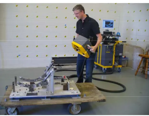
Although the above coordinate measurement technologies may differ, all systems share similarities in data acquisition and data post-processing/alignment methods. Verady, Martin, and Cox (1997) and Wolf, Roller, and Schafer (2000) summarize the application of non-contact measurement technology and how measurement results are generated.

Figure 1. Sample Measurement of Part in Fixture Using 3D Coordinate Metrology

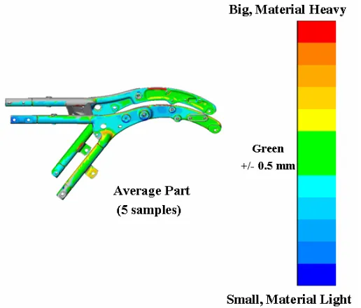
A common output of 3D, non-contact coordinate measurement systems is point cloud or line data along with a color map to show deviation from product design nominal. For multiple measurement samples of the same part, average and range color maps may also be generated. Figure 2 illustrates an Average Color Map for a sample of five frame assembly parts scanned while being held in a conventional part-holding fixture. Of note, the dark blue and dark red colors represent areas with the largest deviation. Furthermore, the cooler, bluish colors suggest that the part is smaller, or material light to design nominal, and the warmer, reddish colors indicate that the part is bigger, or material heavy. The mix of colors depicted in the figure below shows that this part has several off-nominal or mean bias conditions.

Figure 2. Average Color Map for Sample of 5 Panels

Figure 3 illustrates a Range Color Map for the same sample of five parts. For this color map, the range scale goes from green (less than 0.5 millimeters) to red (greater than 2.5

millimeters) in half millimeter increments. The large amount of orange in the color map indicates that the sample of five chosen for this study has significant variation. Of note, we will be

Figure 3. Range Color Map for Sample of 5 Panels

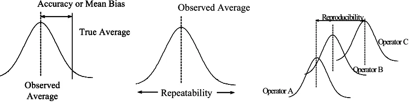
The capability of a measurement system is typically characterized by its accuracy (measured mean values versus true mean values) and various sources of variation error, often categorized as repeatability and reproducibility (AIAG, 2002). A typical decomposition of a measured process mean and variance for a dimension into these measurement error sources is shown in Figure 4.

These sources of measurement system error are further illustrated in Figure 5 and defined by the Automotive Industry Action Group (AIAG, 2002). We now review these terms and implications for 3D, non-contact measurement.

Figure 5. Accuracy, Repeatability, and Reproducibility (Source: AIAG, 2002)

The measurement system accuracy is typically determined by comparing an observed measurement or average from a specific measurement device to a true, or master, reference measurement determined from a more precise gage or set of master parts (See Equation 1). Here, the reference value may be viewed as the standard in which a measurement device is trying to replicate. With 3D, non-contact measurement, accuracy is typically obtained by measuring known artifacts. Measurement system inaccuracies or biases typically result in systematic shifts in reported mean values.

1 Re ferenceValue Equation verage

Observed A t Bias

Measuremen = −

Measurement system repeatability represents the random variation in measurements when one operator uses the same measurement system to measure the same parts multiple times. Repeatability error is often estimated using either Analysis of Variance (ANOVA) or the

Average/Range Method (Montgomery and Runger, 1993). Equation 2 shows the Average/Range Method, which shall be used in this paper.

Observed Average

True Average Accuracy or Mean Bias

Observed Average

True Average Accuracy or Mean Bias

Reproducibility Operator B Operator A Operator C Repeatability Observed Average Observed Average True Average Accuracy or Mean Bias

Observed Average

True Average Accuracy or Mean Bias

1974 , Statistics Industrial and Control Quality A.J., Duncan, see values, of table for appraisers of number x parts of number and trials of number on based constant d t measuremen contact -non 3D for space t measuremen a mapping or fixture a loading as such setup t measuremen part unique a represents trial each where operator same the using trials i of subgroup a for range average 2 Equation / * 2 * 2 = = = R where d R ity repeatabil σ

Repeatability is occasionally separated into the following two categories: static and dynamic. Static repeatability (Equation 3) is often determined by repeatedly measuring the same part in a fixture without loading and unloading the part between measurement trials (or without a new measurement setup for a fixtureless measurement). Dynamic repeatability is typically derived from variance estimates of overall repeatability and static repeatability (Equation 4).

appraisers of number x parts of number and trials of number on based constant d trials between setup without trials i of subgroup a for range average 3 Equation / * 2 * 2 = = = − static static ity repeatabil static R where d R σ 2 2 ity repeatabil static ity repeatabil ity repeatabil

dynamic− = σ −σ −

σ Equation 4

Reproducibility (Equation 5) represents the variation in average measurements made by different operators using the same gage and the same parts. Reproducibility effects often are assigned only after establishing that a statistically significant mean difference relative to the inherent repeatability error exists between operators. For purposes of this study, we have mitigated this potential error source by using one operator to measure all parts.

The study of measurement system repeatability and reproducibility is often referred to as R&R or a Gage R&R Study. Most manufacturers evaluate Gage R&R using ratios or indices that compare the measurement system variation (e.g., σR&R) to the part variation and/or the tolerance

width (Montgomery and Runger, 1993). These indices are intended to represent the error of the complete measurement system, not simply the equipment or physical gage.

To provide an assessment of inherent measurement equipment accuracy, or static repeatability, one typically uses known artifacts such as a highly precise ball bar (Bryan, 1982) or other objects, such as cones or spheres, with known dimensions. One would then measure accuracy and static repeatability based on the measurement system results versus these known artifact dimensions. Although this approach clearly provides the best measure of the pure accuracy and inherent repeatability of a measurement system, it does not necessarily reflect the capability of a measurement system to evaluate production parts under typical manufacturing conditions.

Manufactured part inspection is more complicated, particularly for larger, irregularly shaped, or non-rigid objects, and where one is trying to align measurement results to a global coordinate system and report measurements relative to design nominal product dimensions. Here, measurements are affected by the datum locator scheme and whether a part-holding fixture is used. Other factors that may affect measurement results are operating instructions and skills, particularly for 3D coordinate measurement equipment.

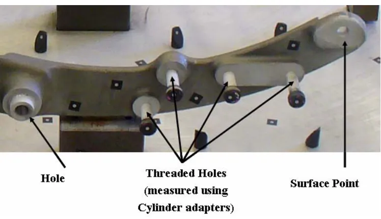
In addition to these systematic sources of measurement error, certain individual features within a part may be more difficult to measure than others. Figure 6 illustrates some common feature types, including surface points, trim edges, and hole size/positional dimensions. Among these, the accuracy, repeatability, and reproducibility errors may differ by feature type or from dimension-to-dimension within a given part. Historically, trim edges and hole/slot/bore positions are more difficult to measure than surface points, particularly for 3D, non-contact measurement systems (Hammett et. al., 2005). Furthermore, some features may not even be directly

Figure 6. Part Feature Types

The practical effect of these differences is that an assessment of measurement system capability requires further breakdown by different feature types. In other words, one cannot assign a single measurement error value that represents every dimension of an entire part. For purposes of this study, we will analyze differences using surface profile points, hole locations, and hole sizes on repeatability and alignment error.

3.0 Common Alignment Methods Used in 3D Coordinate Metrology

The goal of an alignment or registration process is to transform measured part data from a local coordinate system that is internal to the measurement device into a global coordinate

system that the user desires. To do this, measurement operators typically identify the geometric elements in the measured part data that represent the datum set. The operator then transforms the data by mapping each geometric element of the datum set from the measured data to a known dimension in the desired coordinate system.

measured data and their references. Since 3D, non-contact measurement and alignment typically involves more than 6 points to arrest the six degrees of freedom required for dimensional

reporting, alignment solutions may result in virtual interferences.

In the literature, alignment methods are often classified as either iterative or non-iterative and then further subdivided by different assumptions and algorithms5 used to develop a solution (Yau et. al., 2000; Gruen and Acka, 2005). For over-constrained conditions involving many points to match between a local and global coordinate system, most software tools use an iterative method to minimize distance errors between measured points and alignment reference points (e.g., use a variant of the iterative closest point algorithm (Besl and McKay, 1992). In the absence of a perfect mathematical solution (i.e., resolution of all alignment points exactly to their known reference), alignments are solved by successively searching and moving output data to a new position until a final solution is found. Here, the final alignment solution is reached or converges when iterative adjustments become so small that they have no effect on the outcome.

Due to the iterative nature of over-constrained alignment, using the same method with the same set of discrete points may not always produce exactly the same measurement results. For example, software may yield a different solution when the alignment algorithm start point is different. Based on our experiences, such differences are usually negligible.

In many cases, manufacturers rely on the discretion of measurement technicians to determine the most appropriate alignment method/algorithm for a given measurement application, particularly if a certified check fixture is not available. We now discuss some of these generic alignment method options (or families of methods) commonly found in 3D coordinate measurement software. Again, although the exact algorithms used by a software provider are proprietary, most offer at least one of the following generic options6:

• Best Fit Alignment using all available measurement points

• Iterative Closest Point Alignment using Pre-Specified Reference Points • Closed Form, Non-Iterative Alignment based on Fixed Coordinate Points

3.1 Best Fit Alignment

Best Fit is a nonspecific alignment that globally minimizes the distance of every

measured point to its reference, often via an iterative least-square fitting algorithm. Simple, best-fit algorithms provide each measured point essentially the same weight in the alignment

calculation, regardless of its functionality or inherent importance to the product. Thus, suspect or unimportant data points can exert influence on the final result. However, since large-volume metrology involves data collection for millions of points on a part, the effect of any individual point is minuscule.

A best-fit alignment is often used to find the starting point for a more specific alignment method (e.g., iterative closest point based on datum reference points) or as an exploratory tool to examine global relationships between part features. In other words, best fit may be used to get a measured part at least within its proper orientation relative to a part or global coordinate system. Best-fit alignment is typically dominated by the surface profile and ignores resolved features (e.g., since the bulk of measured points are generally on the part form). Rarely will best fit be specific enough to completely resolve a dimensional issue, but it can provide clues for where a user should look next. Finally, results of best-fit alignment methods usually do not reflect the datum reference scheme described in GD&T drawings. As such, one typically cannot assess part dimensional conformance to product specifications based on a best-fit solution.

3.2 Iterative Closest Point (ICP) Alignment using Pre-Specified Reference Points

Iterative Closest Point Alignment (ICP) and related methods (Besl and McKay, 1992; Rusinkiewicz, 2001) use specifically selected features from the resolved geometry to align or register measured data against a nominal reference (e.g. Product CAD data). The iterative alignment is essentially a best fit for a subset of interesting features among the thousands available in a large-volume measurement application.

is maintaining its relationship to its part form. In another example, a user may want to investigate if manufacturing datum locators are consistent with functional locators.

3.3 Closed Form, Non-Iterative Alignment based on Fixed Coordinate Points

Closed form, non-iterative fixed coordinate alignment resolves the geometry of measured features to specific coordinates that the user provides, usually a small subset of points. This is done by solving a closed form solution of absolute orientation using unit quaternions (e.g., see Horn, 1987). The presence of fixture artifacts in a measurement system often prompts a user to apply this type of alignment. Tooling balls, J-corners or other fixed objects that have a known coordinate may be used to create the fixed coordinates. Often, fixed coordinate alignment is done using more than the conventional six degrees of freedom. For instance, one may use four or six tooling balls placed near the physical extremes of a check fixture. Here, one uses a least-squares fitting algorithm to resolve the geometry equal to the desired coordinate.

Resolved geometry that easily decomposes into a set of discrete orthogonal points is a typical candidate for a fixed coordinate alignment. Complex shapes or geometry that is difficult to resolve or decompose may warrant the use of ICP algorithms.

For all of the above alignment methods discussed, numerous variants exist. These variants, often passed along through cascade training practices, are part of the “tricks of the trade” within the metrology community. The purpose of this paper is not to evaluate the accuracy and repeatability for each of the above methods. Rather, we wish to promote the notion that users have options and should quantify, or at least recognize, the potential impact of the alignment method used.

4.0 Quantifying Alignment Error

over-constraints during measurement. In the presence of these over-constraints, a user will typically assess whether a particular alignment method results in a lower root-mean-square measurement error across the alignment features. In other words, if one applies more than six constraints, a high likelihood exists that some points will be in positional conflict, resulting in some measurement error between the resolved alignment points and their nominal specification.

Equation 6 provides a common method for determining the root-mean-square alignment error (σalign-RMS). For 3D coordinate measurements, alignment points must constrain each axis.

Equation 6

A simple example to illustrate potential alignment variation occurs with the usage of tooling balls. If one uses only six alignment points from tooling balls to resolve the six degrees of freedom in 3D coordinate measurement, the root mean square error will be zero (i.e., a perfect fit). Still, if one uses more than six alignment points (e.g., use each individual XYZ dimension from four tooling balls for a total of 12 alignment points), then some measurement error across the alignment points will likely exist. The commonly used analogy to explain this occurrence is that a three-legged stool will resolve into a perfect plane and never wobble, but a fourth leg likely will be outside of this plane unless an adjustment is made to the length of at least one individual leg.

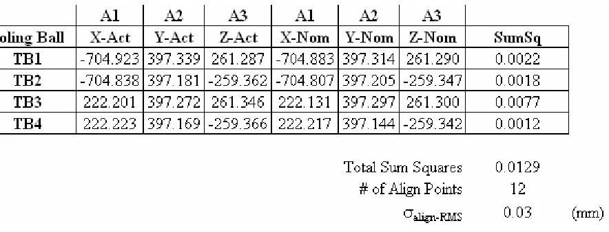
As an example, suppose we have XYZ nominal values for each of four tooling balls from a part-holding fixture (i.e., 12 alignment points). After applying a fixed coordinate alignment for this over-constrained condition, we may record the final measured deviation of each alignment point. Table 1 displays actual and nominal measurements for each tooling ball alignment point from a case study we performed. Using these data, we may obtain a σalign-RMS = 0.03 millimeters,

which is relatively small compared to the tolerances for this part. Of note, this particular example illustrates the worst observed RMS alignment error using check fixture and tooling balls from our case study. The average σalign-RMS across all of our fixed coordinate alignments was 0.02.

Table 1. Alignment Root-Mean-Square Calculation Example

This estimated alignment variation, however, only provides a measure of how well a particular alignment method resolves its constraint measurements to their nominal condition for a particular measurement sample. Thus, one may still have significant alignment differences across multiple trials even when measuring the same exact part, if different alignment methods are used (with potentially different alignment points used). This result may occur even if the σalign-RMS is

zero. To reinforce this point, if one uses only six alignment points, the σalign-RMS =0. However,

the observed mean value for one set of six alignment points may differ significantly from measuring the same part using another set of six. These potential differences in mean values between alignments are a focus of this paper.

Figure 7. Alignment Error

Equation 7

Historically, manufacturers have not measured systematic alignment error. Instead, they either have used the same fixture and alignment method for all measurements to maintain consistent mean biases, or more likely have ignored it, assuming it is not significant. With the rise of 3D, non-contact measurement and related software advancements, numerous alignment options are available. Measurement system operators and data post-processors are using these options to explore different alignments in an effort to produce the most informative part

measurement results. In some cases, setup constraints, such as the desire to measure parts in tools or at a physical location that does not have a holding fixture, require operators to develop an alignment method to fit a particular measurement application. Interestingly, many managers and engineers are not even aware of the potential changes to dimensional results that may occur

trials of number parts of number alignments of number ) .. ( ) .. ( ) * / ( *) / ( 1 1 2 2 2 = = = − = − = r n k where X X Min X X Max X r n d X k k diff diff

align σrepeat

σ

d2* – constant based on sample size, n is # of parts, r is # of trials

based on even small changes to the alignment method used. With this paper, we hope to increase awareness of this issue.

5.0 Alignment Case Study – Frame Section Assembly

In this section, we present a case study of the frame section assembly shown earlier to demonstrate the effects of systematic alignment differences using our proposed alignment error metric. This particular frame assembly was chosen for several reasons. First, the measured part has a part-inspection holding fixture, even though the manufacturer often measures it without using this fixture. For example, depending on the purpose and location of the process

improvement study, some parts are measured using a fixture; others are measured in a free-state condition. Another reason for selecting this part is that the datum locating scheme was heavily debated during design reviews7. Third, the part exhibits high process variation relative to its design tolerances. The median standard deviation among critical features was 0.7 (or

approximately +/- 2.1 millimeters of total variation) relative to typical tolerances of +/- 1.5 millimeters. For parts with such high variability, a natural question is whether this variation is the result of the manufacturing process or the measurement system.

Finally, this part requires the use of more than six alignment points due to its non-rigid nature and has some measurement challenges related to a tendency for the part to twist from side to side. Of note, numerous manufactured parts are aligned with more than six points and have tendencies to twist during restraining, so these represent common measurement challenges.

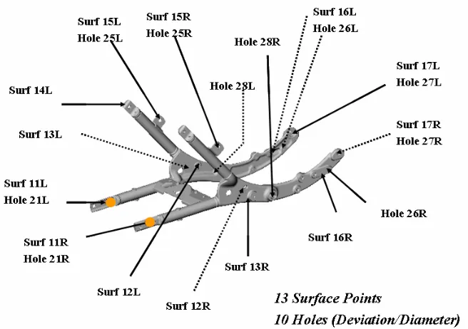
For this measurement system study, five frame assemblies were randomly selected from the manufacturing process. (The samples are shown in Figure 8.) Each part was lightly coated with a powder to reduce the reflectivity of certain shiny machined surfaces for non-contact measurement. The parts were then measured using a white light area scanner generating both a full cloud of points and discrete measurements at 33 key dimensions. Figure 9 illustrates these 33 critical measurement dimensions for this assembly. These dimensions include 13 surface points and 10 holes where both location and diameter are measured.

Figure 8. Frame Section Case Study Sample Measurements

Figure 9. Assembly Dimensions

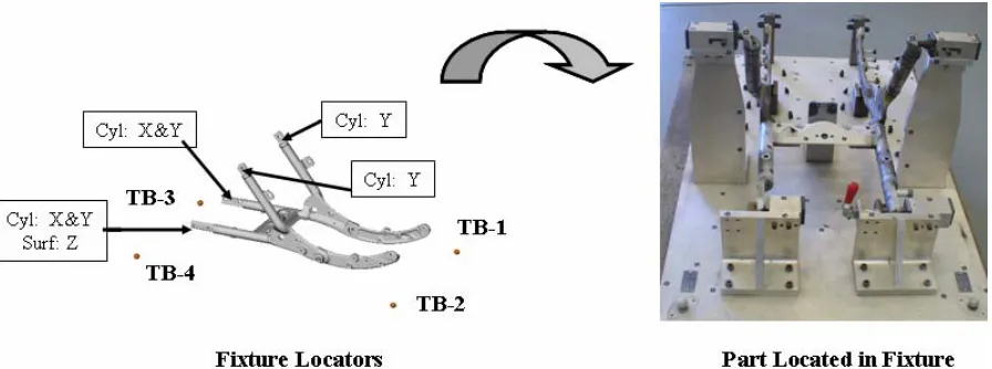
We measured each part assembly using both a holding fixture (as shown in Figure 10) and in a fixtureless, or free-state condition. The holding fixture had four supplier-certified

Figure 10. Frame Section Assembly Holding Fixture and Locating Scheme

Figure 11. Frame Section Case Study Sample Measurements

For this study, three alignment methods were examined based on differences used across measurement applications. The first alignment, Method A, was fixture-based (refer back to Figure 10) and used fixed coordinates alignment based on the four tooling balls and 12 alignment points (X, Y, and Z dimensions for each tooling ball). In terms of locators, this fixture has two regardless-of-feature size (RFS) pins for X and Y, two diamond pins for Y, and one net surface to control X.

The second alignment, Method B, involved fixtureless measurements using an iterative, closest-point alignment algorithm. For this alignment, cylinders were measured at the same four hole locations as used in the holding fixture along with four net surfaces to align the vehicle cross vehicle (Z). The alignment points are shown in Figure 12 below.

Figure 12. Alignment Method B – Iterative Alignment

Of importance to note, for the fixtureless, surface-based locators, we used numerous discrete points on the feature versus relying on a single discrete point (see Figure 13 for

example). This is a common technique with 3D, non-contact measurement for several reasons. First, most fixtures use an actual surface area (e.g., net locator pad) instead of a discrete point to locate the datum surface. Second, some individual discrete points may not compute during post processing and alignment. Having multiple points on the surface helps ensure that the

Figure 13. Multiple Points to Resolve a Locator Surface

A third alignment, Method C, was developed to address a common challenge in

6.0 Alignment Methods and their Impact on Measurement System Variation

In this section, we analyze alignment effects on static repeatability, overall repeatability, and alignment mean differences. To effectively assess mean differences by alignment method, one would prefer that the observed measurement system repeatability is not affected by the part selected for measurement or whether a fixture is used or not. Demonstrating this repeatability consistency is necessary to satisfy the homogeneity of variance assumption desired when using Analysis of Variance (ANOVA) Methods to assess whether mean differences between alignment methods are statistically significant. So, prior to examining alignment mean differences, we first verify that the inherent static repeatability of our measuring equipment is low and that the overall repeatability including load operation and part setup is consistent across different parts and fixture methods.

6.1 Static Repeatability

Historically, static equipment repeatability, which is the ability to repeatedly measure the same part with the same equipment without load/unload or new setup between measurement trials, is often relatively low compared to repeatability when including part setup factors (Hammett, 1999). In other words, the loading or setup of a part during measurement is often a much larger contributor to measurement system repeatability than the equipment itself. To verify this condition for this case study, one of the sample parts (Part #2) was measured three times in the fixture without unloading the part for each of three trials.

Figure 14. Box Plot (Static Repeatability Range versus Overall Repeatability Range)

Figure 15. Static versus Overall Repeatability by Dimensions Type

We may further summarize the part setup effect by computing the average range across all 33 dimensions and converting this to an estimate of overall σstatic-repeatability using equation 3

shown earlier. The results are shown in Table 3.

Table 3. Static versus Dynamic Repeatability (Equipment) Effect

inherently repeatable relative to both the tolerances and the observed part variation 8. When considering the fixture load and setup effects, the average range (including load/setup between trials) is 0.166, which translates to σrepeatability = 0.095. This variation is much greater than the

static repeatability of 0.043. As expected, the dynamic factors represent a statistically significant difference. Since all of these dynamic factors are inherent to part measurement, we will now examine different alignments using the overall repeatability.

6.2 Repeatability - Alignment A versus B

Next, we examine the range for each set of three trials per dimension and part for both Alignment Method A (Fixture with Fixed Coordinates) and Alignment Method B (Fixtureless with Iterative Alignment). Thus, we have 330 total range measurements (33 dimensions x 5 parts x 2 alignments). A histogram of the range outputs is shown in Figure 16.

Figure 16. Histogram of all Repeatability Ranges (based on trials of 3)

8 _{The static repeatability observed in this study, while low relative to the part variation in this particular}

As expected, the distribution of range measurements is skewed right. One reason for this skew is that range measurements are bounded by zero. Still, we may explore whether other factors such as dimension location, part, fixture, or dimension type (i.e., diameter, hole center, or surface) are contributing factors that explain some of this skew. We now investigate each of these potential contributors.

First, we explore whether selection of an individual part or use of fixture has a significant effect on range repeatability across multiple trials. Ideally, these factors should not have a

significant effect. In other words, one should not see a difference in repeatability based on the part randomly selected for measurement or the fixture used. Note, fixture differences may translate to significant mean differences, but the repeatability error should be similar.

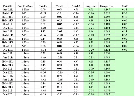
Using a General Linear ANOVA model on our range measurements by Part (or sample) and Fixture (Holding Fixture versus No Holding Fixture), we may observe that no statistically significant difference exists (for alpha = 0.05). Table 4 summarizes the ANOVA analysis, and Figure 17 pictorially shows this consistency using a Multiple Box Plot. We should note that in conducting our study, we re-measured four of the sample measurement trials (out of the 30 Æ 5 parts x 2 alignments x 3 trials each) because of extreme outliers for a few individual dimensions. This approach is similar to the common practice when using average/range method for a Gage Repeatability and Reproducibility study where one must ensure that the trial ranges are stable and consistent before evaluating mean difference effects between operators.

Table 4. Two Factor ANOVA Results: Part and Fixture

Analysis of Variance for Range-Dim, using Adjusted SS for Tests Source DF Seq SS Adj SS Adj MS F P

Part 4 0.03434 0.03434 0.00859 0.66 0.621 Fixture 1 0.00072 0.00072 0.00072 0.06 0.814 Error 324 4.21733 4.21733 0.01302

Total 329 4.25239

Figure 17. Multiple Box Plot

These results represent an important finding necessary to properly evaluate alignment mean differences. In this study, we may surmise that the loading effect for our fixture is comparable in terms of repeatability to the part setup effect when measuring a part without a fixture (assumes a unique mapping with each measurement trial).

This finding may appear counterintuitive at first. Many practitioners would expect a fixture to provide better repeatability than fixtureless measurement. However, for this particular part and fixture design, the load process is such a dominant factor that it negates the potential advantage of applying clamping forces with the holding fixture to consistently stabilize a part for measurement.

Although no statistically significant differences were observed for either the part selected or the fixture effect, clearly some differences exist by type of dimension (diameter, hole center position, or surface). Table 5 summarizes an ANOVA analysis for the range measurements by the three dimension types. As discussed earlier, the range repeatability for a diameter

Although we recognize that differences exist by dimension type and specific discrete point, we note that the same 33 dimensions are used for all parts measured. Thus, for purposes of comparing alignment methods, we treat these particular range differences as random, inherent common cause variation effects when comparing means across different alignment methods.

Table 5. One Way ANOVA Results for Range Measurements by Dimension Type

Source DF SS MS F P Dim Type 2 0.7312 0.3656 33.95 0.000 Error 327 3.5211 0.0108

Total 329 4.2524

S = 0.1038 R-Sq = 17.20% R-Sq(adj) = 16.69%

Next, we compare our repeatability ranges by fixture/alignment method. Table 6 summarizes the repeatability ranges and provides an estimate for σrepeatability per alignment

methods A and B. In this study, the fixture/alignment method exhibited no significant effect on the average repeatability. Both methods yield an average σrepeatability of approximately 0.095

millimeters with an expected range of approximately 0.57 (+/- 3 σrepeatability) across a trial of

three. Given an average part standard deviation of 0.7 across the 33 dimensions, this repeatability error is relatively low (% R&R – Total Variance = 0.0952 / 0.72 = 1.8 %). This finding suggests that the measurement system is clearly discriminating measurement system variation from part variation.

6.3 Repeatability: Alignment A versus B versus C

In this section, we compare alignment methods A and B to a third approach, which we refer to as the Split Iterative, or Alignment Method C. To understand the adoption of this method, we first review the design intent of the GD&T. The desired datum scheme involves creating axes between both the upper and lower functional attachment holes. However, this is difficult to replicate in a conventional holding fixture. In addition, this manufacturer prefers to use regardless-of-feature size pins, which further deviates from the GD&T specified condition.

In using a conventional iterative approach across the full assembly in alignment method B, we were not able to force a parallel axis. Thus, any out-of-perfect alignment condition between the holes essentially averages out when using an iterative approach, which treats each alignment point as a discrete, un-weighted entity.

In an attempt to get the measurement software to create a virtual axis, we split the part into two essentially symmetric sides. We then used applicable locators from each side to align the part independent of the other side. In doing so, we set the two-directional locators to nominal as opposed to averaging them out as done in their normal measurement process involving an over-constrained condition. In addition, we added one cross car locator at the rear of the part for each independent measurement side. The reason is that in using a subset of GD&T datum locators, we needed an additional cross-car constraint to stabilize the part. Furthermore, we wanted this anti-rotational locator at the opposite end of the part to minimize any lever effects of having all the locators at the front of the part. After aligning each independent section, we

digitally assembled the two sides to generate a final part assembly measurement. By forcing each two-directional locator to nominal versus averaging their differences via an iterative method, we were able to effectively create the desired axis.

The repeatability results for all three alignment methods are shown in Table 7 below. Interestingly, the repeatability for Method C, though still higher than the σstatic-repeatability of 0.043

Table 7. Repeatability by Alignment Method

In a deeper interrogation, the primary improvements in range measurements occurred at a few surface point measurements (see Figure 18). Consistent with earlier findings, ranges across trials for diameter measurements were not affected by alignment method.

Figure 18. Range Measurements: Free State versus Split Iterative by Dimension Type

Interestingly, ad hoc methods such as this one are often at the discretion of the measurement operator, particularly advanced metrology specialists. In many cases, engineers and managers are unaware that subtle GD&T interpretations are occurring, particularly when software allows one to easily change settings and alignment methods.

7.0 Alignment Methods and their Impact on Mean Deviations (σalignment)

In this section, we explore mean differences across alignment methods. To do so, we convert the variation in mean differences across dimensions into a new overall measurement system variation metric, σalignment. As mentioned previously, this metric represents differences in

mean values based on the alignment method used. Our main contention is not to suggest that there is only one appropriate alignment strategy, but rather to recognize that differences are inevitably going to exist by application and resource constraints.

Through this report, we hope to convince readers that these differences are significant and that more effort is needed to help develop consistent methods to determine which is indeed the best or most representative. In the following subsections, we first compare mean differences in our fixture-based method versus the fixtureless iterative alignment method. Then, we compare differences with these methods to the split iterative method.

7.1 Alignment Effect: Method A versus B

First, we examine mean differences between alignment methods A and B. Again, the distinctions here are the usage of a holding fixture and a different alignment method. Method A uses the holding fixture with fixed coordinates alignment based on four tooling balls and 12 corresponding alignment points. Method B is based on measuring the part in a fixtureless condition and applying an iterative alignment based on the GD&T intent datum locators.

different across methods, translating to a σalign equal to 0.39 (based on Equation 7). Given that

the σrepeatability was approximately 0.095, this alignment mean difference effect is significant.

Thus, the decision to measure this part using the holding fixture with fixed coordinate alignment versus in a free-state condition with iterative alignment has far greater implications toward making appropriate dimensional corrections than the measurement system repeatability or reproducibility9.

Figure 19. Mean Difference: Alignment Method A versus B

Table 8. Mean Differences by Alignment Method

We further may examine these mean differences by dimension type. As expected, alignment mean differences are much higher for surface and hole center positional dimensions than for hole diameter sizes. Table 9 shows that the average mean difference for hole diameters is only 0.05 millimeters, while more than 0.7 millimeters for surface and hole centers. These differences are illustrated further using Scatter Plots in Figures 20 and 21. Here, we observe relatively low correlation (R2 = 0.32) between the same surface or hole center measurement from one alignment method to another. In contrast, hole measurements, while having much smaller mean differences, are more strongly correlated (R2= 0.7) between alignment methods. Thus, the

selection of alignment method has less impact on reporting diameter size measurements than positional measurements.

Table 9. Range and Mean Differences by Feature Type

Non-Diameter Dimensions

R2 = 0.32

-2 -1.75-1.5 -1.25-1 -0.75-0.5 -0.250 0.250.5 0.751 1.251.5 1.752

-2 -1.8 -1.5 -1.3 -1 -0.8 -0.5 -0.3 0 0.25 0.5 0.75 1 1.25 1.5 1.75 2

A: Fixture - Fixed Coordinates

B

: N

o

F

ixtu

re - I

ter

ati

v

e

Mean Diameter Values (Align A vs. B)

R2 = 0.70

-0.3 -0.2 -0.1 0 0.1 0.2 0.3

-0.3 -0.2 -0.1 0 0.1 0.2 0.3

A: Fixture - Fixed Coord

B

: N

o

F

ixt

u

re

I

terat

iv

e

Figure 21. Scatter Plot of Mean Values by Hole Diameter Dimension

7.2 Alignment Effect: A versus B versus C

Next, we examine alignment mean differences between the split iterative method and the other two methods. Figure 22 shows average color maps for the three alignments. Visually, method B and C look similar. Still, in comparing alignments using our 33 critical dimensions, the differences in means between alignments B and C also are significant (see Table 10). In fact, the average mean difference between Methods B and C was also approximately 0.54 for a σalign =

Figure 22. Alignment A versus B versus C

Table 10. Mean Alignment Differences

The implications of these findings are substantial. We used three different methods based on GD&T intent and found significant mean differences among them. In our view, Method C provided the most representative result because it created an axis between the main process attachment holes per GD&T design intent. However, conventional practice typically regards the fixture method as the master, particularly if done using a CMM.

8.0 Conclusions

From our perspective, the most important takeaway of this study is that alignment really matters! Changing alignments significantly affects mean values even if the repeatability of the alignment schemes is similar. In some cases, different alignment methods may reasonably reflect GD&T intent even though clear differences exist in the mean values of the measurement output across the methods. In many cases, alignment differences are potentially a much greater issue than assessing equipment accuracy or repeatability, where hardware/software providers are often able to meet requirements for various applications.

With advances in coordinate measurement hardware and software, operators have more options to explore different alignment methods. With more options, however, a greater

opportunity exists for systematic alignment differences. Thus, the final selection of an alignment scheme requires an understanding of the data collection purpose and consideration of the

REFERENCES

1. AIAG (2002). Measurement Systems Analysis. Reference Manual. 3rd Edition. Automotive Industry Action Group.

2. American Society of Mechanical Engineers (ASME) (1995). Dimensioning and Tolerancing (ASME Y14.5M-1994 Reaffirmed 1999). New York: Author.

3. Besl P. J., and McKay N. D. (1992). A method for registration of 3d shapes. In IEEE Transactions on PAMI vol. 14, pp. 239–256.

4. Bryan, J.B. (1982). “A simple method for testing measuring machines and machine tools Part 1: Principles and applications,” Precision Engineering, Volume 4, Issue 2, pg 61-69. 5. Chen, F., Brown, G.M., and Song, M. 2000. Overview of three-dimensional shape

measurement using optical methods.Society of Photo-Optical Instrumentation Engineers. 6. Duncan, A.J., (1974). Quality Control and Industrial Statistics, Fourth Edition.

7. Gershon R. and Benady M., (2001). “Non-contact 3-D Measurement Technology Enters a New Era,” Quality Digest, September.

8. Gruen A., and Akca, D. (2005). Least squares 3D surface and curve matching. ISPRS Journal of Photogrammetry and Remote Sensing, Volume 59, Issue 3, May 2005, Pages 151-174

9. Hammett, P. and Baron, J., (1999). Automotive Body Measurement System Capability. Report prepared for the Auto Steel Partnership Program.

10.Hammett, P.C., Garcia Guzman, L., Frescoln, K., and Ellison, S. (2005). “Changing Automotive Body Measurement System Paradigms with 3D Non-Contact Measurement Systems”, Society of Automotive Engineers World Congress, Paper No. 2005-01-0585. 11.Horn, B.K.P., (1987). Closed-form solution of absolute orientation using unit

quaternions, Journal of the Optical Society of America A, Vol, 4, page 629, April 1987 12.Krulikowski, A. (1999). Advanced Concepts of GD&T. Wayne, MI: Effective Training

Inc.

13.Meadows, J. (2009). Geometric Dimensioning and Tolerancing: Applications, Analysis, and Measurement, ASME.

14.Montgomery, D.C., and Runger, G.C., (1993). “Gauge Capability and Designed Experiments Part 1: Basic Methods,” Quality Engineering, 6:1:, pp. 115-135.

15.Rusinkiewicz, S. and Levoy, M., (2001). “Efficient variants of the ICP algorithm,” Third International Conference on 3D Digital Imaging and Modeling.

16.Verady, T., Martin, R. and Cox, J. (1997) “Reverse engineering of geometric models: an introduction,” Computer-Aided Design, Vol. 29, No. 4, pp. 255-268.

17.Wolf, K., Roller, D., and Schafer D., (2000). “An approach to computer-aided quality control based on 3D coordinate metrology,” Journal of Materials Processing Technology, Volume 107, Issues 1-3, Pages 96-110