Stability Analysis in Computational Problems Regarding Power Networks

2018 International Conference on Applied Mechanics, Mathematics, Modeling and Simulation (AMMMS 2018) ISBN: 978-1-60595-589-6

Stability Analysis in Computational Problems Regarding Power Networks

Dan D. MICU*, Levente CZUMBIL, Denisa STET and Andrei CECLAN

Electrical Engineering Faculty, Technical University of Cluj-Napoca, Romania

*Corresponding author

Keywords: Power Systems, Stability analysis, Conditioning, Wielandt-Kantorovich inequality

Abstract. The paper presents a stability analysis of power systems using condition number, eigenvalues and Wielandt-Kantorovitch inequality. The examples are selected from the domain of d.c. electric circuits and power systems. The novelty of the paper is the use of these mathematical tools in this type of practical applications.

Introduction

Small-signal stability analysis is about power systems stability when subject to small disturbances (perturbations in the mathematical model). If the power system oscillations caused by small disturbances can be suppressed, such that the deviation of system state variables remain small for a long time, the power system is stable. If the amplitude of the oscillations continues to increase, the power system is unstable. The power system stability could be affected by many factors, including initial operation conditions, strength of electrical connections among components, characteristics of control devices etc. So, one of the main task in power system analysis is to carry out stability analysis of the equivalent electrical circuits mathematical model in order to assess the power system under specified operating condition. [1]

The Wielandt-Kantorovitch (W-K) method provides a very useful tool for the analysis of power system stability. In the following, we will introduce the mathematical background of this approach.

Perturbation-conditioning-stability in Computational Problems in Power Systems (CP-PS)

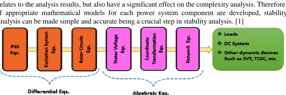
In power system stability analysis, the mathematical models of system components not only directly relates to the analysis results, but also have a significant effect on the complexity analysis. Therefore, if appropriate mathematical models for each power system component are developed, stability analysis can be made simple and accurate being a crucial step in stability analysis. [1]

Figure 1. Steps in mathematical models for stability studies.

are subjected to perturbations. In CP-PS, the cause vectors that could be affected are voltage and current generators and the link matrix elements are permeability, permittivity, conductivity and all any other passive circuit elements. [3]

We will study how the matrix solution process is affected by changes to the computational problem.

The main reason for doing this is to attain an understanding of why some linear system problems which appear in CP-PS are difficult to solve. Usually this involves a concept known as – conditioning.

Condition Number

Singular matrices, as the terminology implies, are perhaps something of a rarity in CP-PS. This does not means that we do not have to worry about them. It can be demonstrate that singular matrices are arbitrarily very close to a nonsingular matrix. The concept of ill-conditioned linear system Az=u is a system for which small perturbations in u lead to large changes in solution z. The quantity that gives information about the nonsingular matrix stability to perturbations is called condition number that depends entirely on the Euclidian norm of the square matrix in the problem, not on the right-side vector, yet it shows up as an amplifier to the relative change in the right-side vector: [4]

n 1 2 1 2 ||A ||

|| A || ) A ( K

   

 

(1)

where 2n

2 2 2

1  ...

 are the eigenvalues of the ATA matrix.

The condition number is a good indicator of how close is a matrix to be singular - the closer a matrix is to being singular, the larger its condition number. It is also very useful in assessing the accuracy of systems solution. Therefore, since the condition number is such an important indicator of how well we can compute with the matrix, it is very useful if it could be easily computed. A condition number estimator is a fairly standard feature of modern linear systems software used in CP-PS.

Stability Study when Perturbation Affects the Cause Vector

In the power systems stability studies is compulsory to establish the relationship between cause (perturbation) and effect (system response). The response of the system under normal operating conditions (in the absence of the perturbation) has to be studied, followed by analysis of the same device where its operation is perturbed.

Considering a linear system Az=u and where the aim is to understand how the solution z changes as the right-side vector u changes. The perturbed system will be Az'= u'. The norm of the variation of this solution calculated for a threshold relative to the norm of the solution will be called immunity (I). Aplying the spectral norm a sufficient condition is obtained, for that z‘ is not perceived as a perturbed vector: [5]

 

u u ' u A K z

z ' z

2 2 2

2    



(2)

This shows that the condition number is a relative error magnification factor. That is, changes in the

u vector can cause changes K(A) times as large in the solution. Therefore, to be able to provide better immunity of the device, the matrix condition number must be reduced. It is noticed that a smaller condition number allows larger perturbations that maintains however, the device in a good compatibility range. If the matrix is ill conditioned - meaning that the condition number is large - then a small change in the data could lead to a large change in the solution.

Stability Study Using Wielandt-Kantorovitch Inequality

The W-K inequality offers a geometrical information regarding the stability of a system affected by a small perturbation. The considered device/system is described by the matrix equation: A z = u.

If the sources are perturbed, the cause vector will be u’ and the solution of the equation (the effect

vector) won’t be z but z’.

Let be β the angle between the vectors z and z’ and φ the angle between vectors u and u’. The W-K inequality is depicted below, where k(A) is the condition number of A matrix:

 

tg or 2

 







' ' ' ' 2 /     

 k u u u u u u u u

tg T T (3)

To demonstrate the utility of the W-K inequality, two devices having a two systems of equations as a mathematical model, are considered:

a) First device:

          21 z 1 . 1 z 2 10 z 0.5 z 2 1 2

1 _{with the computed condition number k(A) =64.59}

b) Second device:           1 . 20 z 01 . 1 z 2 10 z 5 . 0 z 2 1 2

1 _{with the computed condition number k(A) =626.98}

Well-conditioned system, with k(A)=64,59 Ill-conditioned system, with k(A)= 626,98

Figure 1. Angle between vectors.

The increased value of the β angle shows that between solution of system b) before and after the perturbation, it can be a huge difference. In other words the system b) is ill-conditioned, which however satisfies the inequality and is very close to the maximum angle specified by the W-K inequality.

These two examples point to an important fact, namely: a system is ill-conditioned if the angle formed by the vector representing the initial solution z and the perturbed solution z‘ will be higher and closer to the maximum value given by the W-K inequality. It is noted that the condition number of the system b) is about ten times higher than that of the system a). This is translated into a much lower immunity to perturbation of the second device (the ill-conditioned system). The  angle formed by the vectors

u and u‘ is close to the angle made by the corresponding vectors from example a). [5]

Stability Study of a d.c. Electric Circuit Model

The physical model is a d.c. electric circuit with three parallel branches according to Fig. 3:

E1=15[V], R1(x)=x=1,2,3...50[Ω], E2=5[V], R2=20[Ω], E3=10[V], R3=30[Ω]. The E3 source is

The parameter for stability study is the resistance R1=x. A MathCAD algorithm was developed to

complete the mathematical computation and matrix method is used to solve the electrical circuit:

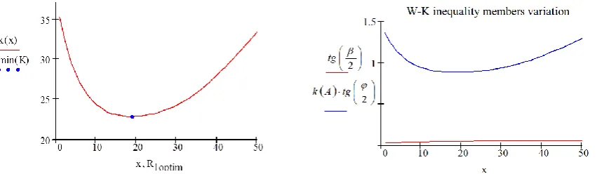
Solving the W-K inequalities it is determined that the minimum of Euclidean condition number

k(19)=22.85 is obtained for x=R1=19[Ω], and the minimum of the right hand side of W-K is 0.877.

For this value of R1, the circuit stability is maximum and the value of I1, the current in the perturbed

branch, is close to zero. A function for the R1(x) value identification is built for which the k(x) of the M matrix take a minimum value so that the circuit is stable for a p perturbation.

Figure 3. Condition number variation. Figure 4. Variation of the Wielandt -Kantorovitch inequality.

The stability of the device for two parameters, x=R1, y=R3 for 1-30[Ω] was also investigated. The

minimum of Euclidean condition number is k=17.98 for R1=R3=9[Ω].

m

n   

 

Valoare k( ) R1optim m R1optim 9  R2optim n R2optim 9 

k Figure 5. R1 and R2 optimum values. Figure 6. Condition number variation.

Stability Study of a Power System Using Eigenvalues Analysis

In power systems applications, eigenvalues and eigenvectors have certain “physical” meanings, depending on the nature of the problem. Typically, the practical interest is the following [6-7]:

 to determine all eigenvalues and corresponding eigenvectors;

 to determine just a specific eigenvalues and corresponding eigenvector (eigenvalue highest or lowest in absolute value, the first few eigenvalues in descending or ascending order of their absolute values);

 to determine the eigenvalues and eigenvectors for real Hermitian matrix;

 to locate the eigenvalues in the complex plane or on the real axis without their explicit calculation.

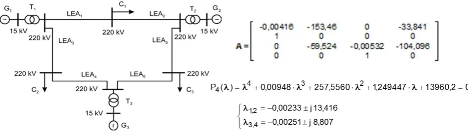
Figure 7. Investigated power network/Eigen values of the coefficients matrix.

The power system is stable when all eigenvalues have negative real part or there are real numbers with negative sign (generators remain in synchronism; the steady state after perturbation is identical to the steady state before perturbation).

The existence of one or more positive real eigenvalues or complex values with positive real part indicates instability (loss of synchronism in asymptotic or oscillatory mode, depending on the nature of the respective eigenvalues). The imaginary part of the complex eigenvalues provide information regarding the natural frequencies of oscillation of the generators in the system.

Related to the investigated network, there are two pairs of complex conjugate eigenvalue having a negative real part. Consequently, the power system is naturally stable at the low intensity perturbation considered. Natural oscillation are of 13.416[rad/s] and 8.807[rad/s], which corresponds to the frequency about 2.14[Hz] (period of 0.47[s]) and 1.40[Hz] (period of 0.71[s]).

Conclusions

The paper demonstrates the possibility of using Euclidian condition number and W-K inequality to study power system stability, when the mathematical model of the network is a system of matrix equations. The main advantage consist in using one single number dependent on the systems structure, to characterize the stability of the network. An original aspect is the use of electrical circuits and a power system configuration to demonstrate and validated the determined numerical techniques.

References

[1]X. F. Wang et al., Modern Power System Analysis, Springer, 2008.

[2]U. Tautenhahn, Regularization of linear ill-posed problems with noisy right hand side and noisy operator, Journal of Inverse and Ill Posed Problems, Vol. 16, No. 5, 2008, pp. 507–524.

[3]H. J. Kim et all, A New Algorithm for Solving Ill-Conditioned Linear Systems, IEEE, Trans. Magn., Vol. 32, No. 3, 1996, pp. 1373–1376.

[4]A. Neubauer, Computation of discontinuous solutions of 2D linear ill-posed integral equations via adaptive grid regularization, Journal of Inverse Problems, Vol. 15, No. 1, 2007, pp. 99–111.

[5]D.D. Micu, A. Ceclan, Numerical Methods, Ed. Mediamira, 2007.

[6]V. V. Vasin, Some approaches to reconstruction of non-smooth solutions of linear ill-posed problems, Journal of Inverse and Ill Posed Problems, Vol. 15, No. 6, 2007, pp. 625–640.