Adaptive bridge estimation for high dimensional regression models

(1)

R E S E A R C H

Open Access

Adaptive bridge estimation for

high-dimensional regression models

Zhihong Chen

1

_{, Yanling Zhu}

1*

_{and Chao Zhu}

2

*_{Correspondence:}

[email protected]

1_{School of International Trade and}

Economics, University of International Business and Economics, Beijing, 100029, P.R. China

Full list of author information is available at the end of the article

Abstract

In high-dimensional models, the penalized method becomes an eﬀective measure to select variables. We propose an adaptive bridge method and show its oracle property. The eﬀectiveness of the proposed method is demonstrated by numerical results.

MSC: 62F12; 62E15; 62J05

Keywords: adaptive bridge; high-dimensionality; variable selection; oracle property; penalized method; tuning parameter

1 Introduction

For the classical linear regression modelY =Xβ+ε, we are interested in the problem of variable selection and estimation, whereY= (y,y, . . . ,yn)Tis the response vector,X= (X,X, . . . ,Xp) = (x,x, . . . ,xn)T_{= (}_xij₎

n×pis ann×pdesign matrix, andε= (ε,ε, . . . ,εn)T

is a random vector. The main topic is how to estimate the coeﬃcients vectorβ∈Rp_when pincreases with sample sizenand many elements ofβequal zero. We can transfer this problem into a minimization of a penalized least squares objective function

ˆ

β=arg min

β Q(β), Q(β) =Y–Xβ

₊_λ

p

j=

|βj|ζ,

where · is thelnorm of the vector,λis a tuning parameter. Forζ> ,βîs called the bridge estimator proposed by Frank and Friedman []. There are two well-known special cases of the bridge estimator. Ifζ= , it is the ridge estimator in Hoerl and Kennard []; if ζ= , it is the Lasso estimator by Tibshirani [], which does not possess the oracle property in Fan and Li []. For  <ζ≤, Knight and Fu [] studied the asymptotic distributions of bridge estimators when the number of covariates is fixed and provided a theoretical jus-tification for the use of bridge estimators to select variables. The bridge estimators can distinguish between the covariates whose coefficients are exactly zero and the covariates whose coefficients are nonzero. There is much statistical literature about penalization-based methods. Some examples include the SCAD by Fan and Li [], the elastic net by Zou and Hastie [], the adaptive lasso by Zou [], the Dantzig selector by Candes and Tao [] and the non-concave MCP penalty by Zhang []. For bridge estimation, Huanget al.[] extended the results of Knight and Fu [] to infinite dimensional parameters and

(2)

showed that for  <ζ<  the bridge estimator can correctly select covariates with nonzero coeﬃcients and under appropriate conditions the bridge estimator enjoys the oracle prop-erty. Subsequently, Wanget al.[] studied the consistency of the bridge estimator for a generalized linear model.

In this paper, we consider the following penalized model:

ˆ

β=arg min

β Q(β), Q(β) =Y–Xβ

₊_λ

p

j=

˜

ωj|βj|ζ, (.)

whereω˜ = (ω˜,ω˜, . . . ,ω˜p)Tis a given vector of weights. Usually, if we let the initial

esti-matorβ˜= (β˜,β˜, . . . ,β˜p)T be the non-penalized MLE, thenω˜j=| ˜βj|–,j= , , . . . ,p.βˆis

called the adaptive bridge estimator. We propose and study the adaptive bridge estimator method (abridge for short). We derive some theoretical properties of the adaptive bridge estimator for the case whenpcan increase to infinity withn. Under some conditions, with the choice of the tuning parameter, we show that the adaptive bridge estimator enjoys the oracle property; that is, the adaptive bridge estimator can correctly select covariates with nonzero coefficients with probability converging to one and that the estimator of nonzero coefficients has the same asymptotic distribution that it would have if the zero coefficients were known in advance.

As far as we know, there is no literature to discuss the properties of an adaptive bridge, so our results make up for this. Compared with the results in Huanget al.[] and Wang

et al.[], the condition (A) (see Section ) imposed on the true coefficients is much weaker. Moreover, in Wanget al.[] one needs the true coefficients to meet the additional condition called covering number. Besides, Huanget al.[] and Wanget al.[] both use the LQA algorithm to obtain the estimator. The shortcoming of the LQA algorithm is that if we delete one variable in some step of the iteration, this variable will have no chance to appear in the final model. In order to improve this algorithm, we employ the MM algorithm to improve the stability.

The rest of the paper is organized as follows. In Section , we introduce notations and assumptions which will be needed in the our results and present the main results. Section  presents some simulation results. The conclusion and the proofs of the main results are arranged in Sections  and .

2 Main results

For convenience of the statement, we ﬁrst give some notations. Letβ= (β,β, . . . ,βp)T

be the true parameter,J={j:βj= ,j= , , . . . ,p},J={j:βj= ,j= , , . . . ,p}, the

car-dinality of the setJ is denoted byqandh=min{|βj|:j∈J}. Without loss of gener-ality, we assume that the ﬁrstqcoeﬃcients of covariates (denoted byX()) are nonzero,

X() be covariates with zero coeﬃcients,β= (β()T ,β()T )T, βˆ= (βˆ()T,βˆ()T)T correspond-ingly. Actually,p,q,X,Y,β, andλare related to the sample sizen, we omitnfor conve-nience. In this paper, we only consider the statistical properties of the adaptive bridge for the case of p<n; consequently we put p=O(nc_), _q ₌_O₍_nc_), _λ₌_O₍_n–δ_{), where}

≤c<c< ,δ> . Here we use the terminology in Zhao and Yu [] , and we deﬁne

ˆ

β=sβif and only ifsgn(βˆ) =sgn(β), where we denote the sign of ap× vectorβ as

(3)

andλmax(Z) the minimum and maximum eigenvalue ofZ, respectively. Denote XT_nX:=D

andD=D D DD

, whereD=_nX()TX().

Next, we state some assumptions which will be needed in the following results.

(A) The error termεis i.i.d. withE(ε) = andE(εk) < +∞, wherek> . For the special

case we denoteE(ε) =σ.

(A) There exists a positive constantMsuch thath≥Mnα, wheremax{–_,c_–,_––ζ}<

α<min{c–δ,c_+–δζ–ζ}andδ+α+

 ζ<c.

(A) Supposeτ and τ are the minimum and maximum eigenvalues of the matrix D.

There exist constantsτandτsuch that <τ≤τ≤τ≤τ, and the eigenvalues

of _nXT_var₍_Y₎_X_{are bounded.}

(A) Letgibe the transpose of theith row vector ofX(), such thatlimn→∞n–_max__≤_i_≤_n_gT i × gi= .

It is worth mentioning that condition (A) is much weaker than those in the literature where it is commonly assumed that the error term has Gaussian tail probability distri-bution. In this paper we allowεto have a heavy tail. The regularity condition (A) is a common assumption for the nonzero coeﬃcients, which can ensure that all important covariates could be included in the ﬁnally selected model. Condition (A) means that the matrix 

nX T

()X()is strictly positive definite. For condition (A), we will use it to prove the asymptotic normality of the estimators of the nonzero coefficients. In fact, if the nonzero coefficients have an upper bound, then we can easily verify condition (A).

2.1 Consistency of the estimation

Theorem .(Consistency of the estimation) If <ζ< ,and conditions(A)-(A)hold,

then there exists a local minimizerβˆof Q(β),such that ˆβ–β=Op(n δ+α–c

ζ _).

Remark . By condition (A), we know thatc–δ–α>  and the estimator consistency refers to the order of sample size and tuning parameter. Theorem . extends the previous results.

2.2 Oracle property of the estimation

Theorem .(Oracle property) If <ζ< ,and conditions(A)-(A)hold,then the adap-tive bridge estimator satisﬁes the following properties.

() (Selection consistency)limn→∞P{ ˆβ=sβ}= ;

() (Asymptotic normality)√ns–uT(βˆ()–β()) d

−→N(, ),wheres=σuTD–ufor

anyq×vectoruandu ≤.

Remark . By Theorems . and ., we can easily see that the adaptive bridge is able to consistently identify the true model.

3 Simulation results

In this section we evaluate the performance of the adaptive bridge estimator proposed in (.) by simulation studies. Setζ = / and simulate the data by the modelY=Xβ+ε, ε∼N(,σ_{), where}_σ_{= ,}_β

()= (–., –., –., , , , –, –, –)T. The design matrix

Xis generated by ap-dimensional multivariate normal distribution with mean zero and a covariance matrix whose (i,j)th component isρ|i–j|_{, where we let}_ρ_{= . and .,}

(4)

Example . The sample sizen=  and the covariates numberp= .

Example . The sample sizen=  and the covariates numberp= .

Example . The sample sizen=  and the covariates numberp= .

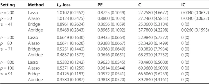
We connect the minorization-maximization (MM) algorithm by Hunter and Li [] and the Newton-Raphson method to estimate the adaptive abridge (abridge), where the tuning parameter is selected by -fold cross-validation. Meanwhile, we compare our results with that from lasso [], adaptive lasso (alasso) and bridge methods. In order to evaluate the performance of the estimators, we select four measures calledL-loss, PE, C, and IC.L -loss is median of ˆβ–βto evaluate the estimation accuracy, and PE is the prediction error deﬁned by median ofn–_Y_–_X_βˆ_{. The other two measures are to qualify the} per-formance of model consistency, where C and IC refer to the average number of correctly selected zero covariates and the average number of incorrectly selected zero covariates. The numerical results are listed in Table  and Table , whereυ equals the number of zero coeﬃcients in the true model and the numbers in parentheses are the corresponding standard deviations which are obtained by  replicates.

[image:4.595.116.481.410.553.2]

Note that in every case the adaptive bridge outperforms the other methods in sparsity, which can select the smaller model. For the adaptive bridge the prediction error is a little higher than the other methods, but when consider the estimation accuracy, the adaptive

Table 1 Simulation results forρ= 0.5

Setting Method L2-loss PE C IC

n= 200

p= 50

υ= 41

Lasso 0.5459 (0.1160) 0.8830 (0.1126) 28.4540 (5.3337) 0 (0) Alasso 0.5442 (0.1149) 0.8790 (0.1099) 28.5300 (5.2421) 0 (0) Bridge 0.4733 (0.1120) 0.8755 (0.1068) 28.2700 (5.0834) 0 (0) Abridge 0.4617 (0.1155) 0.9005 (0.1038) 38.8380 (2.9903) 0 (0)

n= 500

p= 80

υ= 71

n= 800

p= 100

υ= 91

Table 2 Simulation results forρ= 0.9

Setting Method L2-loss PE C IC

n= 200

p= 50

υ= 41

Lasso 1.0102 (0.2452) 0.8725 (0.1049) 27.2580 (4.6677) 0.0040 (0.0632) Alasso 1.0123 (0.2475) 0.8800 (0.1024) 27.2460 (4.5851) 0.0040 (0.0632) Bridge 0.8961 (0.2624) 0.8656 (0.1059) 25.0600 (5.3104) 0 (0) Abridge 0.8468 (0.2843) 0.8965 (0.1092) 37.7800 (4.2298) 0.0260 (0.1593)

n= 500

p= 80

υ= 71

n= 800

p= 100

υ= 91

[image:4.595.117.479.587.732.2]

(5)

bridge is still the winner, followed by bridge. We also ﬁnd the interesting fact that with the sample size nlarger, the performance of correctly selecting the zero covariates for the adaptive bridge is better wheneverρ= . or .. Meanwhile withnincreasing, the estimation accuracy performs better, but the prediction error is worse. Additionally, when ρincreases, the prediction error increases, but the estimation accuracy decreases.

4 Conclusion

In this paper we have proposed the adaptive bridge estimator and presented some theoret-ical properties of the adaptive bridge estimator. Under some conditions, with the choice of the tuning parameter, we have showed that the adaptive bridge estimator enjoys the oracle property. The eﬀectiveness of the proposed method is demonstrated by numerical results.

5 Proofs

Proof of Theorem. In view of the idea in Fan and Li [], we only need to prove that, for any> , there exists a large constantCsuch that

lim inf n→∞ P

inf

u=CQ(β+θu) >Q(β)

≥ –, (.)

which means that with a probability of at least  –there exists a local minimizerβˆin the ball{β+θu:u ≤C}.

First, letθ=n

δ+α–c

ζ _{, then}

Q(β+θu) –Q(β)

=θnuT

XTX n

u–θuTXT(Y–Xβ) +λ

p j= ˜ ωj

|βj+θu|ζ –|βj|ζ

≥λmin

XT_X

n

θnu–nθuTX

T₍_Y_–_X_β

)

n –λ

p

j=

˜

ωj|θ|ζuζ

:=T+T+T, (.)

whereT=λmin(X T_X

n )θnu,T= –nθuT X

T₍_Y_–_X_β

)

n , andT= –λ p

j=ω˜j|θ|ζuζ.

ForT, setv=OP(nα_{) and by assumptions (A) and (A) we have}

PX

T₍_Y_–_X_β_)

n ≥Mv

≤ 

M_vE

_p j=  nX T

j (Y–Xβ) 

= 

nM_vtr



nX

T_var₍_Y₎_X

→ (n→ ∞).

Hence

|T|=

nθuTX

T₍_Y_–_X_β_)

n

≤n|θ|X

T₍_Y_–_X_β_)

n u

(6)

As for |T|, observe that ˜β –β=OP((p_n)/), min|βj| ≤max| ˜βj–βj|+min| ˜βj|, and

assumption (A), we can obtain

=n–αOP

p n

/

+n–αmin| ˜βj|.

This together with assumption (A) yieldsP{min| ˜βj| ≥_Mnα} → (n→ ∞).

Forv=_Mnλpα,P{λ

p

j=ω˜j| ≤v} ≥P{_minλp_{| ˜}_β

j| ≤v}=P{min| ˜βj| ≥

λp

v} → (n→ ∞),i.e., |λ p_j_=ω˜j|=OP(_Mnλpα). Now with assumption (A) we conclude that

|T|=OP

λp Mnα

|θ|ζuζ ₌_O

P()uζ. (.)

When  <ζ <  andCis large enough, by (.) and (.) we see that (.) is determined

byT, so (.) holds.

Proof of Theorem. () First of all, by the K-K-T condition we know thatβˆis the deﬁned adaptive bridge estimator, if the following holds:

⎧ ⎨ ⎩

∂Y–Xβ

∂βj |βj=βˆj=λζω˜j| ˆβj|

ζ–_sgn₍_βˆ

j), βˆj= ,

∂Y–Xβ

∂βj |βj=βˆj≤λζω˜j| ˆβj|

ζ–_, _βˆ

j= .

(.)

Letuˆ=βˆ–βand deﬁneV(u) = nj=(εi–XiTu)+λ p

j=ω˜j|uj+βj|ζ, then we obtain ˆ

u=arg min_uV(u). Notice that n_j_=(εi–XiTu)= –εTXu+nuTDu+εTε, which yields d[ n_j_=(εi–X_iTu)_]

du |u=uˆ = –X

T_ε_{+ }_nD_u_ˆ_{:= }√_n_[_D₍√_n_u_ˆ_{) –}_E_{], where}_E₌X_√Tε

n. Together with

(.) and the fact{|ˆu()|<|β()|} ⊂ {sgn(βˆ()) =sgn(β())}, ifuˆsatisﬁes

D

√

nuˆ()–E()= –λ

√nζW¯() and |ˆu()|<|β()|,

˜

W=ω˜|β|ζ–sgn(β), ω˜|β|ζ–sgn(β), . . . , ω˜p|βp|ζ–sgn(βp) T

,

it follows that|D–

E()|+_λζ√_n|D–W˜()|<

√

n|β()|. DenoteA={|D–|E()+_λζ√_n|D–W˜()|<

√

n|β()|}, we conclude thatP{sgn(βˆ) =sgn(β)} ≥P{A}, from which it follows that

Psgn(βˆ)=sgn(β)≤PAc

≤P

|ξi| ≥

 

√

n|βi|,∃i∈J

+P

λζ

n |Zi|>|βi|,∃i∈J

(7)

where ξ = (ξ,ξ, . . . ,ξq)T =D–E(), Z = (Z,Z, . . . ,Zq)T =D–W(). For I =P{|ξi| ≥

 

√

n|βi|,∃i∈J}, thenE[(ξi)k] <∞,∀i∈J. So its tail probability satisﬁesP{|ξi|>t}= O(t–k_),_∀_t_{> , which yields}

I≤P

|ξi| ≥

 

√

nh,∃i∈J

=qO   √ nh –k

→ (n→ ∞). (.)

ForI, notice that  –I =P{λζ_n|Zi| ≤ |βi|,∃i∈J} and|Zi| ≤ D–W˜() ≤ τ ˜W() ≤

√qhζ–

τminj∈J| ˜βj|, then we can get

 –I≥P

√qλζhζ_–

τminj∈J| ˜βj| ≤nh

=P

λζ≤nτh –ζ



√q minj∈J | ˜

βj|

=  +Op() (n→ ∞).

This follows thatI→ (n→ ∞). Together with (.) and (.),limn→∞P{ ˆβ=sβ}=  holds. This completes the proof of the ﬁrst part of Theorem ..

() Let W = (ω˜| ˆβ|ζ–sgn(βˆ),ω˜| ˆβ|ζ–sgn(βˆ), . . . ,ω˜p| ˆβp|ζ–sgn(βˆp))T, we can easily

get ∂Y–_∂βXβ

j |β=βˆ = ,j∈J, i.e., X

T

()(Y –X()βˆ()) =XT()(X()β()–X()βˆ()+ε) = λζ_W(), which yieldsD(βˆ()–β()) =

XT_()ε

n –

λζ

nW(). It follows from the ﬁrst part of Theorem .

that limn→∞P{D(βˆ()–β()) =

X_()Tε

n –

λζ

nW()}= , then we can see that, for anyq×

vectoruandu ≤,

√

nuT(βˆ()–β()) =n–/uTD–X()Tε– λζ √nu

T_D–

W()+OP(). (.)

Notice that

_λζ√

nu T_D–

W()

≤ λζ

√nτ

ˆβ()ζ–

min_j_∈_J_| ˜βj|

≤λζM

ζ–

 q

ζ–

 _nα(ζ–)–

ζ–_M_τ 

=Onc(ζ–)+α(ζ–)–__,

where the second inequality holds because P{minj∈J| ˆβj| ≥

 Mn

α_{} →}_{ (}_n_{→ ∞}_{), for}

M> . By _c(ζ– ) +α(ζ– ) –_< , we obtain|_λζ√_nuTD–W()|=oP(), which together with (.) yields

√

nuT(βˆ()–β()) =n–/uTD–X()Tε+oP(). (.)

Denotes ₌_σ_uT_D–

u andFi=n– 

s–uTD–

gTi , by assumption (A) and (.) we have

√

ns–uT₍_βˆ

()–β()) = ni=Fiεi+oP()

d

−→N(, ). This completes the proof of the second

part of Theorem ..

Competing interests

The authors declare that they have no competing interests.

Authors’ contributions

All authors contributed equally to the writing of this paper. All authors read and approved the ﬁnal manuscript.

Author details

1_{School of International Trade and Economics, University of International Business and Economics, Beijing, 100029,}

(8)

Acknowledgements

The research was supported by the NSF of Anhui Province (No. 1508085QA13) and the China Scholarship Council.

Received: 16 August 2016 Accepted: 12 October 2016

References

1. Frank, IE, Friedman, JH: A statistical view of some chemometrics regression tools. Technometrics35, 109-148 (1993) (with discussion)

2. Hoerl, AE, Kennard, RW: Ridge regression: biased estimation for nonorthogonal problems. Technometrics12, 55-67 (1970)

3. Tibshirani, R: The lasso method for variable selection in the Cox model. Stat. Med.16, 385-395 (1997)

4. Fan, J, Li, R: Variable selection via nonconcave penalized likelihood and its oracle properties. J. Am. Stat. Assoc.96, 1348-1360 (2001)

5. Knight, K, Fu, WJ: Asymptotics for lasso-type estimators. Ann. Stat.28, 1356-1378 (2000)

6. Zou, H, Hastie, T: Regularization and variable selection via the elastic net. J. R. Stat. Soc., Ser. B67, 301-320 (2005) 7. Zou, H: The adaptive lasso and its oracle properties. J. Am. Stat. Assoc.101, 1418-1429 (2006)

8. Candes, E, Tao, T: The Dantzig selector: statistical estimation whenpis much larger thann. Ann. Stat.35, 2313-2351 (2007)

9. Zhang, C: Nearly unbiased variable selection under minimax concave penalty. Ann. Stat.38, 894-942 (2010) 10. Huang, J, Ma, S, Zhang, CH: Adaptive lasso for sparse high-dimensional regression models. Stat. Sin.18, 1603-1618

(2008)

11. Wang, M, Song, L, Wang, X: Bridge estimation for generalized linear models with a diverging number of parameters. Stat. Probab. Lett.80, 1584-1596 (2010)

12. Zhao, P, Yu, B: On model selection consistency of lasso. J. Mach. Learn. Res.7, 2541-2563 (2006) 13. Hunter, DR, Li, R: Variable selection using MM algorithms. Ann. Stat.33, 1617-1642 (2005)