2019 International Conference on Artificial Intelligence, Control and Automation Engineering (AICAE 2019) ISBN: 978-1-60595-643-5
An Improved Data Assimilation Localization Method Based on Fuzzy
Logic Control
Yu-long BAI*, Irtaza SHAHID, Xiao-yan MA and Yue WANG
College of Physics and Electrical Engineering, Northwest Normal University, Lanzhou 730070, China
*Corresponding author
Keywords: Ensemble transform Kalman filter, Fuzzy Logic control, Covariance fuzzy, Fuzzy
analysis.
Abstract. To determine the best estimates of the ocean or atmospheric state, Data Assimilation (DA) is a methodology to combine all available information from numerical models and observation information. With small ensemble numbers in the Ensemble Kalman filter, the more effective utilization the observation data are, the higher the assimilation performance become. In this study, we proposed a new fuzzy control-based data assimilation system, named FA (fuzzy analysis) and CF (covariance fuzzy), which coupled with fuzzy logic control algorithms to improve assimilation performance. A number of numerical experiments are designed using a classical nonlinear model (the Lorenz-96 model) to explore the effects of the new algorithms on the ensemble transform matrices. The experiments show that the FA algorithm can be selected when the system is in weak assimilation, whereas both algorithms can be implemented in medium assimilation situations. If the system is strongly assimilated, the CF algorithm has demonstrated more robust performance.
Introduction
Data assimilation refers to continue integration the new observation information to obtain the optimal estimation of the current state, which can improve the model forecast accuracy and reduce uncertainty and describe as accurately as possible the true state of the atmosphere, sea and land surface [1]. It has a wide range of applications in atmospheric, oceanic, geophysical and nonlinear dynamical systems. Ensemble Kalman filter (EnKF) is an advanced method that uses several ensembles of model states to propagate and update the estimates of the state covariance[2]. Realistic data assimilation problems are usually implemented with small ensembles to reduce the computational cost. However, using small ensembles can cause a lot of problems, such as rank-deficient with forecast/background ensemble and important Monte Carlo sampling errors [3,4], as well as the ubiquitous nonlinearity of the dynamics system. Several auxiliary techniques have been proposed to alleviate these problems, among others include covariance inflation and local analysis. A number of localisation methods for further improvements have been explored [4]. Although these algorithms to improve the assimilation effect, to avoid the false correlation between observed variables and status updates, in practice, due to the different choices, these algorithms need to be improved. Thus, a data assimilation method of coupled fuzzy algorithm is firstly proposed in [5], which proved the effectiveness of the FETKF (Fuzzy Ensemble Transform Kalman Filter) method with the high-dimensional chaotic Lorenz-96 model. Compared to the former algorithms, it can significantly improve the filtering accuracy in the assimilation system.
Theoretical Background
Ensemble Transform Kalman Filter. he Ensemble transform Kalman filter (ETKF) method was originally put forward by Bishop in [6]. In the formulation, it is expressed that multiply the forecast perturbation by a transform matrix to obtain the analysis perturbation. The ETKF update equations are commonly written as follows:
( )
i i i i
f f
a H x
i i i
x x K y . (1)
,: ,: i
a f
i i
A A T (2)
where all superscript i represented local, xia is the state analysis at ithtime; xif is the state
forecast at ith time; yi is local vector of observations; ,: i
i
K is the local Kalman gain at ith
row; Hi is the local observation operator; Aai,:is theithrow of the analysis perturbed matrix; Afi,:
is theithrow of the forecast perturbed matrix; Ti is the local ensemble transform matrix. The Kalman gain and the Ensemble transform matrix can be expressed as follows:
1/2
/ 1
i i
i i
f
S R H A m (3)
1 1/ 2
,: ,: ( ) / 1
i i i
i i
f T T
i i
K A S IS S R m . (4)
1/ 2
( )
i
i i
T
T IS S . (5)
Where m is the ensemble number, Si are the local ensemble anomalies, and the superscript i
indicates localisation, which will be used to update the ith state variable ; Ri is diagonal, the local observation error covariance Matrix; I is the identity matrix; superscript “T” denotes matrix transposition.
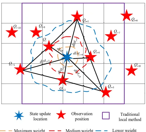
The Principle of Fuzzy Logic Control. The concept of Fuzzy Logic Control was proposed by Zadeh in [7]. To obtain better assimilation effect, we use a new localisation method of coupling the fuzzy logic control. The data assimilation system coupled with fuzzy logic control is comprised of principal blocks as follow:
Normally, fuzzy logic control includes fuzzy variable, fuzzy sets and fuzzy membership functions. In this paper, a set of fuzzy conditions (if…then…) is used to describe the mapping relationship between the Euclidean distance and the weight of the observation point and the state update grid point to obtain the weight of each observation point. The following is the principle of constructing equivalent observation weights using fuzzy theory.
State update location
Observation position
Traditional local method
[image:3.595.178.416.69.285.2]Maximum weight Medium weight Lower weight
Figure 1. Diagram of assimilation system coupled with the fuzzy logic control between observation position and status.
2
2
1 20
i i i j j
dist O V O V i, j , , . (6)
Where OiandOjare the abscissa and ordinate of observation points respectively, Viand Vjare the abscissa and ordinate of state update points respectively. It can be seen from the graph that
i
dist represents the Euclidean distance between the ithobservation point and the ithstate update point, the observation weights can decreases with the distance increases.
In this paper, the fuzzy subset of the input variable "dist" is divided into {the nearest distance, second closest distance..., second farthest distance, farthest distance}, which abbreviated as {I I1, 2,...,I20}. After input quantification, the domain of "dist" isD[0, 20]. The fuzzy subset of the output "coeffs" is {highest weight, higher weight... the second lowest weight, lowest weight}, which is abbreviated as{ ,O O1 2,...,O20}, and its domain isC[0,1]. The connectivity between input fuzzy variable is input fuzzy set and output fuzzy variable is output fuzzy set is represented by a fuzzy implication relation,
( , )
M dist coeffs
coeffs
dist
1
O O2 …
j
O … Om
1
I … … … …
2
I … … … …
… … … …
i
I … … … … …
… … … …
n
I … … … …
where dist{ ,I I1 2,..., }In D,coeffs{ ,O O1 2,...,Om}CandM dist coeffs( , ) denotes the strength
of fuzzy relation for distIi andcoeffsOj, satisfying the implication between input fuzzy
variable is input fuzzy set and output fuzzy variable is output fuzzy set.
Different implication functions are used in the direct use to describe the fuzzy if-then connectivity. In this paper, the well-known Mamdani implication relations is used to illustrate the principle of
) , (Ii Oj
where “
” refers to the Cartesian product of the fuzzy vector. It is a matrix multiplication operator (not a fuzzy operator). According to fuzzy logic control theory, a fuzzy set of equivalent observation weights "coeffs" can be obtained when the fuzzy subsets of input variables "dist" and fuzzyrelationship matrix M complete the fuzzy inference. Thus, the final control variable (output fuzzy variable) can be written as:
coeffsdist M (8)
where is a max-min compositional operation, which is similar to matrix multiplication operation with summation replaced by maximum and product replaced by minimum operators.We employ the maximum membership degree principle in the defuzzification process, the maximum membership degree principle can be written as:
1 2 20
i
j
i i j i , j , , O i O j
coeffs inf Max coeffs dist M ,coeffs dist M . (9)
An Improved Localisation Method Based on Fuzzy Logic Control. Compared with the
orginal LA algorithm, Fuzzy Analysis (FA) gives an approximation of the background error covariance that has completed fuzzy control for each updated state vector element. The fuzzy updating process of the lthstate variable is the same with the above LA algorithm process the covariance with fuzzy control algorithms as follows:
1 1 11 1 1 1
1 1
n
m m m n mn
coeffs x x p coeffs x x p
C P
coeffs x x p coeffs x x p
(10)
The modified matrix CPwill involve in assimilation operations as the background error covariance matrix; Using fuzzy control methods, these improved approaches seek to eliminate the distanced spurious correlations between the state variables in the background error covariance matrix and to improve the quality of the background error covariance matrix.
Numerical Tests
The Lorenz-96 Model. In numerical tests section, we describe experiments with the 40-variable Lorenz-96 model. The coupled set of ordinary differential equations as follows:
1 2 1
( )
i
i i i i
dx
x x x x F
dt (11)
This equation applied for t0, and i1:m, with m40and periodic boundary conditions. The model parameters are chosen to be identical to those of [4]. F is a forcing term that can be tuned to produce chaotic behavior for a given model dimension. In this study, we set F=8.
Figure 2. RMSE values of the LETKF and FLETKF algorithm in the Lorenz-96 model.
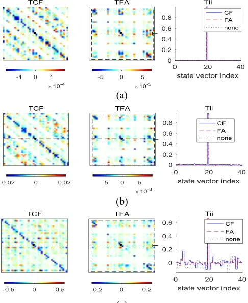
Influence of CF and FA on the Ensemble Transform Matrices. In this section, the proposed
new algorithms CF and FA are demonstrated the effectiveness on the ensemble transform matrix(T). In terms of the EnSRF assimilation process for the three cases with observation errorsRof 10, 1, and 0.001, respectively, the ensemble transform matrices from these two algorithms are extracted for analysis. The results corresponding to the three cases are shown in Figs.3a, 3b and 3c respectively. The ensemble transform matrices of CF is abbreviated as TCF; The ensemble transform matrices of FA is abbreviated as TFA; and the ensemble transform matrix of the 40-th state variables using the three types of algorithms (i.e., no localisation (none), CF and FA) is abbreviated as Tii.
(a)
(b)
(c)
Figure 3.The contrast of the CF and FA algorithms on ensemble transform matrix (T). (a) the observation errors R selected sets 10, the intensity of assimilation is called “weak assimilation”. (b) the observation errors R selected sets 1,
[image:5.595.178.421.373.670.2]with the CF algorithm, the FA algorithm updates the T only for the center point of the defined domain, and other T of non-central elements are not updated. Thus, the FA algorithm performs an asynchronous updating process on T, whereas the CF algorithm performs a synchronous updating process on T; 3) According to Fig. 3(a) , the ensemble transform matrices Tii following updates using the CF and FA algorithms on the same state variable are approximately equal, and the difference between the two algorithms is negligible.
When R = 1, the intensity of assimilation is called “medium assimilation”. As seen in Fig.3(b): 1) The transform matrix TCF from the CF algorithm retains its symmetry and the FA algorithm has little influence; 2) Under medium assimilation, differences gradually emerge in the ensemble transform matrix following updates by the CF and FA algorithms on the same state variable.
When R = 0.001, the intensity of assimilation is called “strong assimilation”. As seen in Fig. 3(c): 1) The ensemble transform matrix TCF of the CF algorithm retains its symmetry. Compared with the case observation error:R= 1, the transform matrix from the FA algorithm is sparse; 2) With an increase of assimilation intensity, which will cause divergence of the two algorithms (i.e., CF and FA), differences in the ensemble transform matrix appear more obvious; 3) According to Fig. 3(c), the difference of the ensemble transform matrix Tii gradually increases following updates by the two algorithms on the same state variable.
Summary
This paper introduces two common processing methods for the covariance matrix. Specifically, the fuzzy control algorithm is coupled to form the new algorithms CF and FA. In the simulation experiments, the paper explores the effects of the CF and FA algorithms on the ensemble transform matrix. Overall, the FA algorithm can be selected when the system is in weak assimilation, whereas both algorithms can be implemented in medium assimilation situations. If the system is strongly assimilated, the CF algorithm has demonstrated more robust performance.
Acknowledgement
This work is supported by the NSFC (National Natural Science Foundation of China) project (grant number: 41861047 and 41461078) and Northwest Normal University young teachers' scientific research capability upgrading program (NWNU-LKQN-17-6).
References
[1]Rolf H. Reichle. Data assimilation methods in the Earth science, J. Advances in Water Resource. 31(2008)1411-1418.
[2] Evensen, G. Data Assimilation:The Ensemble Kalman Filter. Springer, 2006, pp. 279.
[3] Anderson, J. L. Exploring the need for localisation in ensemble data assimilation using a hierarchical ensemble filter, J. Physica D Nonlinear Phenomena. 230(2007):99-111.
[4] Sakov P, Bertino L. 2011. Relation between two common localisation methods for the EnKF. Computational Geosciences, J. 15(2):225-237.
[5] Lu Yongnan, Bai Yulong, Xu Baoxiong, et al. Observation error handling methods of data assimilation coupled with fuzzy control algorithms, J. Remote Sensing Technology and Application.32(2017): 459-465.(In Chinese)
[6] Bishop CH, Etherton BJ, Majumdar SJ (2001) Adaptive Sampling with the Ensemble Transform Kalman Filter. Part I: Theoretical Aspects, J. Monthly Weather Review. 129:420-436.