R E V I E W
Open Access
Extragradient subgradient methods for
solving bilevel equilibrium problems
Tadchai Yuying
1, Bui Van Dinh
2, Do Sang Kim
3and Somyot Plubtieng
1,4**Correspondence: [email protected]
1Department of Mathematics,
Faculty of Science, Naresuan University, Phitsanulok, Thailand
4Center of Excellence in Nonlinear
Analysis and Optimization, Faculty of Science, Naresuan University, Phitsanulok, Thailand Full list of author information is available at the end of the article
Abstract
In this paper, we propose two algorithms for finding the solution of a bilevel equilibrium problem in a real Hilbert space. Under some sufficient assumptions on the bifunctions involving pseudomonotone and Lipschitz-type conditions, we obtain the strong convergence of the iterative sequence generated by the first algorithm. Furthermore, the strong convergence of the sequence generated by the second algorithm is obtained without a Lipschitz-type condition.
MSC: 47J25; 65K10; 65K15; 90C25
Keywords: Bilevel equilibrium problems; Extragradient Subgradient-Halpern methods; Armijo line search; Strong convergence
1 Introduction
LetCbe a nonempty closed convex subset of a real Hilbert spaceH, and letf andgbe bifunctions fromH×HtoRsuch thatf(x,x) = 0 andg(x,x) = 0 for allx∈H. The equi-librium problem associated withgandCis denoted byEP(C,g) : Findx∗∈Csuch that
gx∗,y≤0 for everyy∈C. (1)
The solution set of problem (1) is denoted byΩ. The equilibrium problem is very impor-tant because many problems arise in applied areas such as the fixed point problem, the (generalized) Nash equilibrium problem in game theory, the saddle point problem, the variational inequality problem, the optimization problem and others.
The basic method for solving the monotone equilibrium problem is the proximal method (see [14,16,19]). In 2008, Tran et al. [25] proposed the extragradient algorithm for solving the equilibrium problem by using the strongly convex minimization problem to solve at each iteration. Furthermore, Hieu [9] introduced subgradient extragradient meth-ods for pseudomonotone equilibrium problem and the other methmeth-ods (see the details in [1,8,10,15,17,22,28]).
In this paper, we consider the equilibrium problem whose constraints are the solution sets of equilibrium problems (bilevel equilibrium problems) : Findx∗∈Ωsuch that
fx∗,y≥0 for everyy∈Ω. (2)
The solution set of problem (2) is denoted byΩ∗. The bilevel equilibrium problems were introduced by Chadli et al. [4] in 2000. This kind of problems is very important and inter-esting because it is a generalization class of problems such as optimization problems over equilibrium constraints, variational inequality over equilibrium constraints, hierarchical minimization problems, and complementarity problems. Furthermore, the particular case of the bilevel equilibrium can be applied to a real word model such as the variational in-equality over the fixed point set of a firmly nonexpansive mapping applied to the power
control problem of CDMA networks which were introduced by Iiduka [11]. For more on
the relation of bilevel equilibrium with particular cases, see [7,12,21].
Methods for solving bilevel equilibrium problems have been studied extensively by many authors. In 2010, Moudafi [20] introduced a simple proximal method and proved the weak convergence to a solution of problem (2). In 2014, Quy [23] introduced the algorithm by combining the proximal method with the Halpern method for solving bilevel monotone equilibrium and fixed point problem. For more details and most recent works on the meth-ods for solving bilevel equilibrium problems, we refer the reader to [2,5,24]. The authors considered the method for monotone and pseudoparamonotone equilibrium problem. If a bifunction is more generally monotone, we cannot use the above methods for solving bilevel equilibrium problem, for example, the pseudomonotone property.
Inspired by the above work, in this paper, we propose a method for finding the solution
for bilevel equilibrium problems wheref is strongly monotone andgis pseudomonotone
and Lipschitz-type continuous. Firstly, we obtain the convergent sequence by combining an extragradient subgradient method with the Halpern method. Second, we obtain the
convergent sequence without Lipschitz-type continuity on bifunctiongby combining an
Armijo line search with the extragradient subgradient method.
2 Preliminaries
LetCbe a nonempty closed convex subset of a real Hilbert spaceH. Denote thatxnx
andxn→xare the weak convergence and the strong convergence of a sequence{xn}tox,
respectively. For everyx∈H, there exists a unique elementPCxdefined by
PCx=inf
x–y:y∈C.
It is also known thatPCis a nonexpansive mapping fromHontoC, i.e.,PC(x) –PC(y) ≤ x–y ∀x,y∈H. For everyx∈Handy∈C, we have
x–y2≥ x–PCx2+y–PCx2 and x–PCx,PCx–y ≥0.
A bifunctionψ:H×H→Ris called:
(i) β-strongly monotone onCif
ψ(x,y) +ψ(y,x)≤–βx–y2 ∀x,y∈C;
(ii) monotone onCif
(iii) pseudomonotone onCif
ψ(x,y)≥0⇒ψ(y,x)≤0, ∀x,y∈C.
It is easy to check that the monotone bifunction implies the pseudomonotone bifunction. On the other hand, if the bifunction is pseudomonotone, then we cannot guarantee that the bifunction is monotone, for example, letφ(x,y) =2y–x1–x for allx,y∈R. It follows thatφis pseudomonotone onR+\ {0}butφis not monotone onR+\ {0}. Letψ(x,·) be convex for
everyx∈H. For each fixedx∈H, the subdifferential ofψ(x, .) atx, denoted by∂2ψ(x,x),
is defined by
∂2ψ(x,x) =
w∈H:ψ(x,y) –ψ(x,x)≥ w,y–x ∀y∈H
=w∈H:ψ(x,y)≥ w,y–x ∀y∈H, (3)
studied in [13]. In this paper, we consider the bifunctionsf andg under the following conditions.
Condition A
(A1) f(x,·)is convex, weakly lower semicontinuous and subdifferentiable onHfor every fixedx∈H.
(A2) f(·,y)is weakly upper semicontinuous onHfor every fixedy∈H. (A3) f isβ-strongly monotone onH.
(A4) For eachx,y∈H, there existsL> 0such that
w–v ≤Lx–y, ∀w∈∂2f(x,x),v∈∂2f(y,y).
(A5) The functionx→∂2f(x,x)is bounded on the bounded subsets ofH.
Condition B
(B1) g(x,·)is convex, weakly lower semicontinuous, and subdifferentiable onHfor every fixedx∈H.
(B2) g(·,y)is weakly upper semicontinuous onHfor every fixedy∈H. (B3) gis pseudomonotone onCwith respect toΩ, i.e.,
gx,x∗≤0, ∀x∈C,x∗∈Ω.
(B4) gis Lipschitz-type continuous, i.e., there are two positive constantsL1,L2such
thatg(x,y) +g(y,z)≥g(x,z) –L1x–y2–L2y–z2,∀x,y,z∈H.
(B5) gis jointly weakly continuous onH×Hin the sense that, ifx,y∈Hand
{xn},{yn} ∈Hconverge weakly toxandy, respectively, theng(xn,yn)→g(x,y)as
n→+∞.
Example2.1 Let f,g:R×R→Rbe defined byf(x,y) = 5y2– 7x2+ 2xyandg(x,y) =
Remark2.3 Let the bifunctionf satisfy Assumption A and the bifunctiongsatisfy B. IfΩ=
∅, then the bilevel equilibrium problem (2) has a unique solution, see the details in [23].
Lemma 2.4([6]) Let C be a nonempty closed convex subset of a real Hilbert space H and
φ:C→Rbe a convex,lower semicontinuous,and subdifferentiable function on C.Then
x∗ is a solution to the convex optimization problemmin{φ(x) :x∈C}if and only if0∈
∂φ(x∗) +NC(x∗),where∂φ(·)denotes the subdifferential ofφand NC(x∗)is the normal cone
of C at x∗.
Lemma 2.5([27]) Let{an}be a sequence of nonnegative real numbers,{αn}be a sequence
in(0, 1),and{ξn}be a sequence inRsatisfying the condition
an+1≤(1 –αn)an+αnξn ∀n≥0,
where∞n=0αn=∞andlim supn→∞ξn≤0.Thenlimn→∞an= 0.
Lemma 2.6([18]) Let{an}be a sequence of real numbers that does not decrease at infinity,
in the sense that there exists a subsequence{anj}of{an}such that
anj<anj+1 for all j≥0.
Also consider the sequence of integers{τ(n)}n≥n0 defined,for all n≥n0,by
τ(n) =max{k≤n|ak<ak+1}.
Then{τ(n)}n≥n0is a nondecreasing sequence verifying
lim
n→∞τ(n) =∞,
and,for all n≥n0,the following two estimates hold:
aτ(n)≤aτ(n)+1 and an≤aτ(n)+1.
Lemma 2.7 Suppose that f isβ-strongly monotone on H and satisfies(A4).Let0 <α< 1, 0≤η≤1 –α,and0 <μ<2Lβ2.For each x,y∈H,w∈∂2f(x,x),and v∈∂2f(y,y),we have
(1 –η)x–αμw–(1 –η)y–αμv ≤(1 –η–ατ)x–y,
whereτ = 1 –1 –μ(2β–μL2)∈(0, 1].
Proof Letx,y∈H,w∈∂2f(x,x), andv∈∂2f(y,y). Thus
(1 –η)x–αμw–(1 –η)y–αμv
≤(1 –η)(x–y) –αμ(w–v)
=(1 –η–α)(x–y) +α(x–y) –μ(w–v)
Sincef:H×H→Risβ-strongly monotone,w∈∂2f(x,x), andv∈∂2f(y,y), we have
–βx–y2≥f(x,y) +f(y,x)≥–x–y,w–v. (5)
From (5) and (A4), we have
(x–y) –μ(w–v)2=x–y2– 2μ x–y,w–v+μ2w–v2
≤ x–y2– 2μβx–y2+μ2L2x–y2 =1 – 2μβ+μ2L2x–y2.
This implies that
(x–y) –μ(w–v)≤1 – 2μβ+μ2L2x–y. (6)
By using (4) and (6), we can conclude that (1 –η)x–αμw–(1 –η)y–αμv
≤(1 –η–α)x–y+α1 – 2μβ+μ2L2x–y
= (1 –η–ατ)x–y,
whereτ= 1 –1 –μ(2β–μL2)∈(0, 1].
3 The extragradient subgradient Halpern methods
In this section, we propose the algorithm for finding the solution of a bilevel equilibrium
problem under the strong monotonicity off and the pseudomonotonicity and
Lipschitz-type continuous conditions ong.
Algorithm 1
Initialization: Choosex0∈H, 0 <μ<2Lβ2, the sequences{αn} ⊂(0, 1),{ηn}, and{λn}are
such that ⎧ ⎪ ⎪ ⎨ ⎪ ⎪ ⎩
limn→∞αn= 0,
∞
n=0αn=∞,
0≤ηn≤1 –αn ∀n≥0, limn→∞ηn=η< 1,
0 <λ≤λn≤λ<min(2L11,2L12).
Setn= 0 and go to Step 1.
Step 1. Compute
yn=arg miny∈C
λng(xn,y) +
1 2y–xn
2
,
zn=arg miny∈C
λng(yn,y) +
1
2y–xn
2
.
Step 2. Computewn∈∂2f(zn,zn) and
xn+1=ηnxn+ (1 –ηn)zn–αnμwn.
Theorem 3.1 Let bifunctions f and g satisfy ConditionAand ConditionB,respectively. Assume thatΩ=∅.Then the sequence{xn}generated by Algorithm1converges strongly to
the unique solution of the bilevel equilibrium problem(2).
Proof Under assumptions of two bifunctionsf andg, we get the unique solution of the
bilevel equilibrium problem (2), denoted byx∗. Step 1: Show that
zn–x∗ 2
≤xn–x∗ 2
– (1 – 2λnL1)xn–yn2– (1 – 2λnL2)yn–zn2. (7)
The definition ofynand Lemma2.4imply that
0∈∂2
λng(xn,y) +
1
2y–xn
2
(yn) +NC(yn).
There arew∈∂2g(xn,yn) andw¯ ∈NC(yn) such that
λnw+yn–xn+w¯= 0. (8)
Sincew¯ ∈NC(yn), we have
¯w,y–yn ≤0 for ally∈C. (9)
By using (8) and (9), we obtainλn w,y–yn ≥ xn–yn,y–ynfor ally∈C. Sincezn∈C,
we have
λn w,zn–yn ≥ xn–yn,zn–yn. (10)
It follows fromw∈∂2g(xn,yn) that
g(xn,y) –g(xn,yn)≥ w,y–yn for ally∈H. (11)
By using (10) and (11), we get
λn
g(xn,zn) –g(xn,yn)
≥ xn–yn,zn–yn. (12)
Similarly, the definition ofznimplies that
0∈∂2
λng(yn,y) +
1
2y–xn
2
(zn) +NC(zn).
There areu∈∂2g(yn,zn) andu¯∈NC(zn) such that
λnu+zn–xn+u¯= 0. (13)
Sinceu¯∈NC(zn), we have
By using (13) and (14), we obtainλn u,y–zn ≥ xn–zn,y–znfor ally∈C. Sincex∗∈C,
we have
λn
u,x∗–zn
≥xn–zn,x∗–zn
. (15)
It follows fromu∈∂2g(yn,zn) that
g(yn,y) –g(yn,zn)≥ u,y–zn for ally∈H. (16)
By using (15) and (16), we get
λn
gyn,x∗
–g(yn,zn)
≥xn–zn,x∗–zn
. (17)
Sincex∗∈Ω, we haveg(x∗,yn)≥0. If follows from the pseudomonotonicity ofgonCwith
respect toΩthatg(yn,x∗)≤0. This implies that
xn–zn,zn–x∗
≥λng(yn,zn). (18)
Sincegis Lipschitz-type continuous, there exist two positive constantsL1,L2such that
g(yn,zn)≥g(xn,zn) –g(xn,yn) –L1xn–yn2–L2yn–zn2. (19)
By using (18) and (19), we get
xn–zn,zn–x∗
≥λn
g(xn,zn) –g(xn,yn)
–λnL1xn–yn2–λnL2yn–zn2.
From (12) and the above inequality, we obtain 2xn–zn,zn–x∗
≥2xn–yn,zn–yn–λnL1xn–yn2–λnL2yn–zn2. (20)
We know that
2xn–zn,zn–x∗
=xn–x∗ 2
–zn–xn2–zn–x∗ 2
,
2 xn–yn,zn–yn=xn–yn2+zn–yn2–xn–zn2.
From (20), we can conclude that zn–x∗
2
≤xn–x∗ 2
– (1 – 2λnL1)xn–yn2– (1 – 2λnL2)yn–zn2.
Step 2: The sequences{xn},{wn},{yn}, and{zn}are bounded.
Since 0 <λn<a, wherea=min(2L11,2L12), we have
(1 – 2λnL1) > 0 and (1 – 2λnL2) > 0.
It follows from (7) and the above inequalities that
By Lemma2.7and (21), we obtain
xn+1–x∗=ηnxn+ (1 –ηn)zn–αnμwn–x∗+ηnx∗–ηnx∗+αnμv–αnμv
=(1 –ηn)zn–αnμwn– (1 –ηn)x∗+αnμv+η
xn–x∗
–αnμv
≤(1 –ηn)zn–αnμwn–
(1 –ηn)x∗–αnμv +ηnxn–x∗+αnμv
≤(1 –ηn–αnτ)zn–x∗+ηnxn–x∗+αnμv ≤(1 –ηn–αnτ)xn–x∗+ηnxn–x∗+αnμv
= (1 –αnτ)xn–x∗+αnμv
= (1 –αnτ)xn–x∗+αnτ
μv
τ
, (22)
wherewn∈∂2f(zn,zn) andv∈∂2f(x∗,x∗). This implies that
xn+1–x∗≤maxx n–x∗,
μv
τ
.
By induction, we obtain
xn–x∗≤maxx 0–x∗,
μv
τ
.
Thus the sequence{xn}is bounded. By using (21), we have{zn}, and using Condition (A5),
we can conclude that{wn}is also bounded.
Step 3: Show that the sequence{xn}converges strongly tox∗.
Sincex∈Ω∗, we havef(x∗,y)≥0 for ally∈Ω. Thusx∗ is a minimum of the convex functionf(x∗,·) over Ω. By Lemma2.4, we obtain 0∈∂2f(x∗,x∗) +NΩ(x∗). Then there existsv∈∂2f(x∗,x∗) such that
v,z–x∗≥0 for allz∈Ω. (23)
Note that
x–y2≤ x2– 2 y,x–y for allx,y∈H. (24)
From Lemma (2.7) and (24), we obtain xn+1–x∗
2
=ηnxn+ (1 –ηn)zn–αnμwn–x∗ 2
=(1 –ηn)zn–αnμwn–
(1 –ηn)x∗–αnμv
+ηn
xn–x∗
–αnμv 2
≤(1 –ηn)zn–αnμwn–
(1 –ηn)x∗–αnμv
+ηn
xn–x∗ 2
– 2αnμ
v,xn+1–x∗
≤(1 –ηn)zn–αnμwn–
(1 –ηn)x∗–αnμv
+ηn
xn–x∗ 2
– 2αnμ
v,xn+1–x∗
≤(1 –ηn–αnτ)zn–x∗+ηnxn–x∗ 2
– 2αnμ
v,xn+1–x∗
≤(1 –ηn–αnτ)zn–x∗ 2
+ηnxn–x∗ 2
– 2αnμ
v,xn+1–x∗
≤(1 –ηn–αnτ)xn–x∗ 2
+ηnxn–x∗ 2
– 2αnμ
v,xn+1–x∗
= (1 –αnτ)xn–x∗ 2
+ 2αnμ
v,x∗–xn+1
.
It follows that
xn+1–x∗ 2
≤(1 –αnτ)xn–x∗ 2
+ 2αnμ
v,x∗–xn+1
. (25)
Let us consider two cases.
Case 1: There existsn0such that{xn–x∗}is decreasing forn≥n0. Therefore the limit
of sequence{xn–x∗}exists. By using (21) and (25), we obtain
0≤xn–x∗2–zn–x∗2
≤– αnτ 1 –ηn
zn–x∗ 2
– 2αnμ 1 –ηn
v,xn+1–x∗
+ 1
1 –ηn
xn–x∗2
–xn+1–x∗ 2
. (26)
Sincelimn→∞ηn=η< 1,limn→∞αn= 0 and the limit of{xn–x∗}exists, we have
lim
n→∞xn–x ∗2
–zn–x∗ 2
= 0. (27)
From 0 <λn<aand inequality (7), we get
(1 – 2a)xn–yn2≤(1 – 2λnL1)xn–yn2≤xn–x∗ 2
–zn–x∗ 2
.
By using (27), we obtainlimn→∞xn–yn= 0. Next, we show that lim sup
n→∞
v,x∗–xn+1
≤0. (28)
Take a subsequence{xnk}of{xn}such that
lim sup n→∞
v,x∗–xn+1
=lim sup k→∞
v,x∗–xnk
.
Since{xnk}is bounded, we may assume that{xnk}converges weakly to somex¯∈H. There-fore
lim sup n→∞
v,x∗–xn+1
=lim sup k→∞
v,x∗–xnk
=v,x∗–x¯. (29)
Sincelimn→∞xn–yn= 0 andxnk x¯, we haveynkx¯. SinceCis closed and convex, it is also weakly closed and thusx¯∈C. Next, we show thatx¯∈Ω. From the definition of
{yn}and Lemma2.4, we obtain
0∈∂2
λng(xn,y) +
1
2xn–yn
2
There existw¯∈NC(yn) andw∈∂2g(xn,yn) such that
λnw+yn–xn+w¯= 0. (30)
Sincew¯ ∈NC(yn), we have ¯w,y–yn ≤0 for ally∈C. From (30), we obtain
λn w,y–yn ≥ xn–yn,y–yn for ally∈C. (31)
Sincew∈∂2g(xn,yn), we have
g(xn,y) –g(xn,yn)≥ w,y–yn for ally∈H. (32)
Combining (31) and (32), we get
λn
g(xn,y) –g(xn,yn)
≥ xn–yn,y–yn for ally∈C. (33)
Takingn=nkandk→ ∞in (33), the assumption ofλnand (B5), we obtaing(x¯,y)≥0 for
ally∈C. This implies thatx¯∈Ω. By inequality (23), we obtain v,x¯–x∗ ≥0. It follows from (29) that
lim sup n→∞
v,x∗–xn+1
≤0. (34)
We can write inequality (25) in the following form: xn+1–x∗2≤(1 –αnτ)xn–x∗2–αnτ ξn,
whereξn=2τμ v,x∗–xn+1. It follows from (34) thatlim supn→∞ξn≤0. By Lemma2.5, we can conclude thatlimn→∞xn–x∗2= 0. Hencexn→x∗asn→ ∞.
Case 2: There exists a subsequence{xnj}of{xn}such thatxnj–x∗ ≤ xnj+1–x∗for all j∈N. By Lemma2.6, there exists a nondecreasing sequence {τ(n)} of Nsuch that
limn→∞τ(n) =∞, and for each sufficiently largen∈N, we have
xτ(n)–x∗≤xτ(n)+1–x∗ and xn–x∗≤xτ(n)+1–x∗. (35)
Combining (22) and (35), we have xτ(n)–x∗≤xτ(n)+1–x∗
≤(1 –ητ(n)–ατ(n)τ)zτ(n)–x∗+ητ(n)xτ(n)–x∗+ατ(n)μv. (36)
From (21) and (36), we get
0≤xτ(n)–x∗–zτ(n)–x∗≤– ατ(n)τ
1 –ητ(n)
zτ(n)–x∗+ ατ(n)μ
1 –ητ(n)
v. (37)
Sincelimn→∞αn= 0,limn→∞ηn=η< 1,{zn}is bounded, and (37), we havelimn→∞(xτ(n)–
x∗–zτ(n)–x∗) = 0. It follows from the boundedness of{xn}and{zn}that
lim
n→∞xτ(n)–x ∗2
–zτ(n)–x∗ 2
By using the assumption of{λn}, we get the following two inequalities:
1 – 2λτ(n)L1> 1 – 2aL1> 0 and 1 – 2λτ(n)L2> 1 – 2aL2> 0.
From (7), we obtain
zτ(n)–x∗2≤xτ(n)–x∗2– (1 – 2λτ(n)L1)xτ(n)–yτ(n)2
– (1 – 2λτ(n)L2)yτ(n)–zτ(n)2 ≤xτ(n)–x∗
2
– (1 – 2aL1)xτ(n)–yτ(n)2
– (1 – 2aL2)yτ(n)–zτ(n)2.
This implies that
0 < (1 – 2aL1)xτ(n)–yτ(n)2+ (1 – 2aL2)yτ(n)–zτ(n)2
≤xτ(n)–x∗ 2
–zτ(n)–x∗ 2
.
It follows from (38) and the above inequality that
lim
n→∞xτ(n)–yτ(n)= 0 and n→∞limyτ(n)–zτ(n)= 0. (39)
Note thatxτ(n)–zτ(n) ≤ xτ(n)–yτ(n)+yτ(n)–zτ(n). From (39), we have
lim
n→∞xτ(n)–zτ(n)= 0. (40)
By using the definition ofxn+1and Lemma2.7, we obtain
xτ(n)+1–xτ(n)=ητ(n)xτ(n)+ (1 –ητ(n))zτ(n)–ατ(n)μtτ(n)–xτ(n)
=(1 –ητ(n))zτ(n)–ατ(n)μtτ(n)
–(1 –ητ(n))xτ(n)–ατ(n)wτ(n) –ατ(n)wτ(n) ≤(1 –ητ(n))zτ(n)–ατ(n)tτ(n)
–(1 –ητ(n))xτ(n)–ατ(n)wτ(n) +ατ(n)wτ(n) ≤(1 –ητ(n)–ατ(n)τ)zτ(n)–xτ(n)+ατ(n)wτ(n) ≤ zτ(n)–xτ(n)+ατ(n)wτ(n),
wheretτ(n)∈∂2f(zτ(n),zτ(n)) andwτ(n)∈∂2f(xτ(n),xτ(n)). Sincelimn→∞αn= 0, the
bounded-ness of{wτ(n)}and (40), we havelimn→∞xτ(n)+1–xτ(n)= 0. As proved in the first case,
we can conclude that
lim sup n→∞
v,x∗–xτ(n)+1
=lim sup k→∞
v,x∗–xτ(n)
Combining (25) and (35), we obtain
xτ(n)+1–x∗2≤(1 –ατ(n)τ)xτ(n)–x∗2+ 2ατ(n)μ
v,x∗–xτ(n)+1
≤(1 –ατ(n)τ)xτ(n)+1–x∗2+ 2ατ(n)μ
v,x∗–xτ(n)+1
.
By using (35) again, we have xn–x∗
2
≤xτ(n)+1–x∗ 2
≤2μ τ
v,x∗–xτ(n)+1
. (42)
From (41), we can conclude thatlim supn→∞xn–x∗2≤0. Hencexn→x∗ asn→ ∞.
This completes the proof.
4 The extragradient subgradient methods with line searches
In this section, we introduce the algorithm for finding the solution of a bilevel equilibrium problem without the Lipschitz condition for the bifunctiong.
Algorithm 2
Initialization: Choosex0∈C, 0 <μ<2Lβ2,ρ∈(0, 2),γ ∈(0, 1), the sequences{λn},{ξn},
and{αn} ⊂(0, 1) such that
⎧ ⎨ ⎩
limn→∞αn= 0,
∞
n=0αn=∞,
∞
n=0αn2<∞, λn∈[λ,λ]⊂(0,∞), ξn∈[ξ,ξ]⊂(0, 2).
Setn= 0, and go to Step 2.
Step 1. Compute
yn=arg miny∈C
λng(xn,y) +
1 2y–xn
2
.
Ifyn=xn, then setun=xnand go to Step 4. Otherwise, go to Step 2.
Step 2. (Armijo line search rule) Findmas the smallest positive integer number satisfying ⎧
⎨ ⎩
zn,m= (1 –γm)xn+γmyn,
g(zn,m,xn) –g(zn,m,yn)≥2ρλnxn–yn2.
Setzn=zn,mandγn=γm.
Step 3. Choosetn∈∂2g(zn,xn) and computeun=PC(xn–ξnσntn) whereσn=g(ztnn,x2n)
Step 4. Computewn∈∂2f(un,un) and
xn+1=PC(un–αnμwn).
Setn=n+ 1, and go back to Step 1.
Lemma 4.1([26]) Suppose that yn=xnfor some n∈N.Then the line search corresponding
Lemma 4.2([26]) Let g:Θ×Θ→ ∞be a bifunction satisfying conditions(B1)on C and (B5)onΘ,whereΘis an open convex set containing C.Letx¯,y¯∈Θand{xn},{yn}be two
sequences inΘconverging weakly tox¯,y¯∈Θ,respectively.Then,for anyε> 0,there exist
η> 0and nε∈Nsuch that
∂2g(xn,yn)⊂∂2g(x¯,y¯) + ε ηB
for all n≥nε,where B denotes the closed unit ball in H.
Lemma 4.3([8]) Let the bifunction g satisfy assumption(B1)on C×C, (B5)onΘ×Θ. Suppose that{xn}is a bounded sequence in C,ρ> 0and{yn}is a sequence such that
yn=arg miny∈C
g(xn,y) + ρ
2y–xn
2
.
Then{yn}is also bounded.
Theorem 4.4 Let the bifunction f satisfy ConditionAand g satisfy Conditions(B1)–(B3) and(B5).Assume thatΩ=∅.Then the sequences{xn}generated by Algorithm2converge
strongly to the unique solution of the bilevel equilibrium problem(2).
Proof Letx∗be the unique solution of the bilevel equilibrium problem (2). Then we have x∗∈Ωand there existsv∈∂2f(x∗,x∗) such that
v,z–x∗≥0 for allz∈Ω. (43)
Step 1: Show that
un–x∗ 2
≤xn–x∗ 2
–ξn(2 –ξ2)
σntn
2
. (44)
By the definition ofun, we have
un–x∗ 2
≤PC(xn–ξnσntn) –PC
x∗2
≤xn–ξnσntn–x∗2
=xn–x∗ 2
– 2ξnσn
tn,xn–x∗
+ξnσntn
2
. (45)
Sincetn∈∂2g(zn,xn) andg(zn,·) is convex onC, we haveg(zn,x∗) –g(zn,xn)≥ tn,x∗–xn.
It follows that
tn,xn–x∗
≥g(zn,xn) –g
zn,x∗
. (46)
Sincegis pseudomonotone onCwith respect toΩ, we haveg(zn,x∗)≤0. It follows from
(46) and the definition ofσnthat
tn,xn–x∗
Combining (45) with (47), we obtain un–x∗
2
≤xn–x∗ 2
– 2ξnσn
σntn2
+ξnσntn
2
=xn–x∗2– 2ξn
σntn
2
+ξn2
σntn
2
=xn–x∗ 2
–ξn(2 –ξn)
σntn
2
.
Step 2: The sequences{xn},{yn},{un}, and{wn}are bounded.
Sinceξn∈[ξ,ξ]⊂(0, 2) and (44), we have
un–x∗≤xn–x∗. (48)
By the definition ofxn+1, we get
xn+1–x∗=PC(un–αnμwn) –PC
x∗
≤un–αnμwn–x∗ ≤un–x∗
–αnμ(wn–v) –αnμv
=un–x∗
–αnμ(wn–v)+αnμv. (49)
From Lemma2.7, (48), and (49), we can conclude that xn+1–x∗= (1 –αnτ)un–x∗+αnμv
≤(1 –αnτ)xn–x∗+αnτ
μv
τ
. (50)
This implies that
xn+1–x∗≤max
xn–x∗, μv
τ
.
By induction, we obtain
xn–x∗≤max
x0–x∗, μv
τ
.
Thus the sequence{xn}is bounded. Hence we can conclude from (48) and Lemma4.3
that{yn}and{un}are bounded, respectively. From condition (A4), we have{wn}is also
bounded.
Step 3: We show that if there is a subsequence{xnk}of{xn}converging weakly tox¯and
limk→∞(σnktnk) = 0, then we havex¯∈Ω.
Firstly, we will show that{tnk}is bounded. Since{zn}is bounded, there is a subsequence
{znk}of{zn}converging weakly toz¯By using Lemma4.2, for anyε> 0, there existη> 0 andk0such that
∂2g(znk,xnk)⊂∂2g(z¯,x¯) +
for all k≥k0. Since {tnk} ∈∂2g(znk,xnk), we have{tnk} is bounded. Next, we show that
xnk–ynk →0. Without loss of generality, we can assume thatxnk=ynkfor allk∈N. By Lemma4.1, we obtaing(znk,xnk) > 0 andtnk = 0. Sincelimk→∞(σnktnk) = 0 and{tnk}is bounded, we have
lim
k→∞g(znk,xnk) =k→∞lim
σnktnk
tnk= 0. (51)
It follows from the convexity ofg(znk,·) that
γnkg(znk,ynk) + (1 –γnk)g(znk,xnk)≥g(znk,znk) = 0.
This implies that
γnk
g(znk,xnk) –g(znk,ynk) ≤g(znk,xnk). (52)
By the Armijo line search, we get 2ρλ
nxn–yn
2≤g(z
nk,xnk) –g(znk,ynk), and (52) implies that
ργnk 2λnk
xn–yn2≤γnk
g(znk,xnk) –g(znk,ynk) ≤g(znk,xnk). (53)
Combining (51) with (53), we obtain
lim
k→∞γnkxn–yn
2= 0. (54)
Then we consider two cases.
Case 1.lim supk→∞γnk > 0. There existγ¯> 0 and a subsequence of{γnk}denoted again by{γnk}such thatγnk>γ¯ for allk. So we get from (54) that
lim
k→∞xnk–ynk= 0. (55)
Sincexnkx¯and (55), we haveynk x¯. On the other hand, by the definition ofynk, we have
λnk
g(xnk,y) –g(xnk,ynk)
≥ xnk–ynk,y–ynk for ally∈C. (56)
Therefore
λnk
g(xnk,y) –g(xnk,ynk)
≥–xnk–ynky–ynk for ally∈C.
Lettingk→ ∞in the above inequality, using (55) and the jointly weak continuity ofg, we haveg(x¯,y) –g(x¯,x¯)≥0 for ally∈C. So,g(x¯,y)≥0 for ally∈C. Hencex¯∈Ω.
Case 2.lim supk→∞γnk= 0. From the boundedness of{yn}, there exists{ynk} ⊆ {yn}such that ynk y¯. Let{mk}be the sequence of the smallest non-negative integers such that znk= (1 –γ
mk)x
nk+γ
mky
nkand
g(znk,xnk) –g(znk,ynk)≥
ρ
2λnk
xnk–ynk
Sinceγmk→0, we havem
k> 0. It follows from the Armijo line search that, formk– 1, we
havez¯nk= (1 –γ
mk–1)x
nk+γ
mk–1y
nk and
g(z¯nk,xnk) –g(z¯nk,ynk) <
ρ
2λnk
xnk–ynk
2. (57)
On the other hand, by the definition ofyn, we have
λn
g(xn,y) –g(xn,yn)
≥ xn–yn,y–yn for ally∈C. (58)
Lettingn=nkandy=xnk in (58), we get –λnkg(xnk,ynk)≥ xnk–ynk
2. (59)
Combining (57) with (59), we obtain
g(z¯nk,xnk) –g(z¯nk,ynk) < –
ρ
2g(xnk,ynk). (60)
Sincexnk x¯,ynky¯, andγnk →0, we havez¯nkx¯. From (60) andgis jointly weakly continuous on H×H, we get –g(x¯,y¯) < –ρ2g(x¯,y¯). Sinceρ∈(0, 2), we haveg(x¯,y¯)≥0. Takingk→ ∞in (59), we obtainlimk→∞xnk–ynk= 0. By Case 1, it is immediate that
¯
x∈Ω.
Step 4: Show that the sequence{xn}converges strongly tox∗. By using the definition of
xn+1and (44), we obtain
xn+1–x∗2 =PC
un–αnμwn–PC
x∗2
≤un–αnμwn–x∗ 2
=un–x∗ 2
– 2αnμ
wn,un–x∗
+αnμwn
2
≤xn–x∗ 2
–ξn(2 –ξn)
σntn
2
– 2αnμ
wn,un–x∗
+αnμwn
2
≤xn–x∗2–
σntn
2
– 2αnμ
wn,un–x∗
(61)
+αnμwn
2
.
Settingan=xn–x∗2. It follows from the boundedness of{wn}and{un}that
wn,un–x∗≤M
1 and wn2≤M2. (62)
Combining (61), (62) with the definition ofan, we get
an+1–an+
σntn
2
≤2αnμM1+α2nμ2M2. (63)
Let us consider two cases.
Case 1: There existsn0such that{an}is decreasing forn≥n0. Therefore the limit of{an}
αn, we have
lim n→∞
σntn
= 0. (64)
By the definitions ofxn+1andun, we obtain
un–xn2 =PC(xn–σntn) –PC(xn) ≤ xn–σntn–xn
=σntn. (65)
It follows thatlimn→∞un–xn2= 0, which implies that
lim n→∞un–x
∗2
=a. (66)
Since{un} ⊆Cis bounded, there exists a subsequence{unk}of{un}that converges weakly to someu¯∈Cand satisfies the equality
lim inf n→∞
un–x∗,v
= lim
k→∞
unk–x
∗,v.
Sinceunk u¯∈Cand (43), we have
lim inf n→∞
un–x∗,v
= lim
k→∞
unk–x
∗,v=u¯–x∗,v≥0. (67)
Sincewn∈∂2f(un,un),v∈∂2f(x∗,x∗) andf isβ-strongly monotone onC, we have
wn,x∗–un
≤fun,x∗
≤–βun–x∗2–f
x∗,un
= –βun–x∗2–
un–x∗,v
.
This implies that wn,un–x∗ ≥βun–x∗2+ un–x∗,v. Combining (66), (67) with the
above inequality, we get
lim inf n→∞
wn,un–x∗
≥βa. (68)
Assume thata> 0. Chooseε=12βa. There existsn0such that
un–x∗,wn
≥βa–ε=1
2βa for alln≥n0.
It follows from (61) and the above inequality thatan+1–an≤–αnμβa2+α2nμM2. Summing
this inequality fromn0ton, we obtain
an+1–an0≤–μβa 2
n
k=n0
αk+μM2 n
k=n0
αn2. (69)
Since∞k=n0αk=∞and
∞
k=n0α 2
n<∞, we can conclude from (69) thatlim infn→∞an=
Case 2: There exists a subsequence{anj}of{an}such thatanj≤anj+1 for allj∈N. Let
{τ(n)}be a nondecreasing sequence defined in Lemma2.6. Thus
aτ(n)≤aτ(n)+1 and an≤aτ(n)+1. (70)
From (63) and the definition ofαn, we have lim
n→∞στ(n)tτ(n)= 0. (71)
By the definition ofuτ(n), we obtain
uτ(n)–xτ(n)2 =PC(xτ(n)–στ(n)tτ(n)) –PC(xτ(n)) ≤ xτ(n)–στ(n)tτ(n)–xτ(n)
=στ(n)tτ(n). (72)
This implies thatlimn→∞uτ(n)–xτ(n)2= 0. Since{xτ(n)}is bounded, there exists a
subse-quence{xτ(n)k} ⊆ {xτ(n)}such thatxτ(n)k x¯∈Cand thusuτ(n)k x¯∈C. From (71) and Step 3 of this proof, we getx¯∈Ω. Next, we will show thatuτ(n)k →x
∗. It follows from (61)
that
2ατ(n)kμ
wτ(n)k,uτ(n)k–x
∗≤a
τ(n)k–aτ(n)k+1–
στ(n)ktτ(n)k
2
+ατ(n)kμwτ(n)k
2
≤(ατ(n)kμ)
2M 2.
This implies that
wτ(n)k,uτ(n)k–x
∗≤ατ(n)kμM2
2 . (73)
Sincef isβ-strongly monotone onCandwτ(n)∈∂2f(uτ(n)k,uτ(n)k), we have
x∗–uτ(n)k,wτ(n)k
≤fuτ(n)k,x
∗≤–βu
τ(n)k–x
∗2
–fx∗,uτ(n)k
.
It follows from (73) and the above inequality that uτ(n)k–x
∗2 ≤ 1
β
wτ(n)k,uτ(n)k–x
∗–fx∗,u
τ(n)k
≤ 1 β
ατ(n)kμM2
2 –f
x∗,uτ(n)k
. (74)
Takingk→ ∞, by usinguτ(n)kx¯andατ(n)k→0, we get
lim sup k→∞
uτ(n)
k–x
∗2
≤–fx∗,x¯≤0.
Thereforelimk→∞uτ(n)k–x
∗2= 0. Then, it is easy to see thatlim
n→∞uτ(n)–x∗2= 0.
By the definition ofxn+1, we have
xτ(n)+1–x∗≤uτ(n)–ατ(n)μwτ(n)–x∗
Since{wτ(n)}is bounded, and from the definition ofατ(n), we havelimn→∞xτ(n)+1–x∗2=
0. This means that limn→∞aτ(n)+1= 0. It follows from (50) that limn→∞an= 0. Hence
limn→∞xn–x∗2= 0. This completes the proof.
5 Numerical examples
LetH=RnandC={x∈Rn: –5≤x
i≤5,∀i∈ {1, 2, . . . ,n}}. Let the bifunctiong:Rn×
Rn→Rbe defined by
g(x,y) = Px+Qy,y–x for allx,y∈Rn,
wherePandQare randomly symmetric positive semidefinite matrices such thatP–Qis
positive semidefinite. Thengis pseudomonotone onRn. Indeed, letg(x,y)≥0 for every
x,y∈Rn, we have
g(y,x)≤g(x,y) +g(y,x) = Px+Qy,y–x+ Py+Qx,x–y
= –(P–Q)(x–y),x–y≤0.
Next, we obtain thatgis Lipschitz-type continuous withL1=L2=12P–Q. Indeed, for
eachx,y,z∈Rn,
g(x,y) +g(y,z) –g(x,z) = Px+Qy,y–x+ Py+Qz,z–y– Px+Qz,z–x
=(P–Q)(x–y),y–z
≥–2P–Q
2 x–yy–z
≥–P–Q
2 x–y
2–P–Q
2 y–z
2,
whereP–Qis the spectral norm of the matrixP–Q, that is, the square root of the largest eigenvalue of the positive semidefinite matrix (P–Q)T(P–Q). It is easy to check
thatΩ=∅. Furthermore, we define the bifunctionf :Rn×Rn→Ras
f(x,y) = Ax+By,y–x for allx,y∈Rn,
withAandBbeing positive definite matrices defined by
B=NTN+nIn and A=B+MTM+nIn,
whereM,Nare randomlyn×nmatrices andInis the identity matrix. Then we havef is
n-strongly monotone onRn. Indeed, letx,y∈Rn, we get
f(x,y) +f(y,x) = Ax+By,y–x+ Ay+Bx,x–y
= –(A–B)(x–y),x–y
= –MTM+nIn(x–y),x–y
= –MTM(x–y),x–y–nIn(x–y),x–y
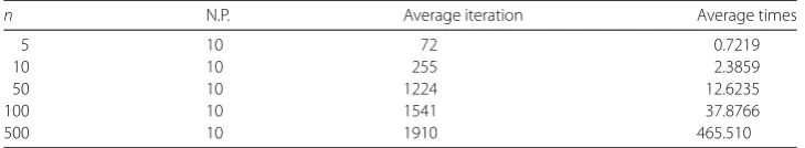
Table 1 The results computed on Algorithm1
n N.P. Average iteration Average times
5 10 72 0.7219
10 10 255 2.3859
50 10 1224 12.6235
100 10 1541 37.8766
500 10 1910 465.510
= –M(x–y)2–nx–y2
≤–nx–y2.
Moreover,∂2f(x,x) ={(A+B)x}and(A+B)x– (A+B)y ≤ A+Bx–yfor allx,y∈Rn.
Thus the mappingx→∂2g(x,x) is bounded andA+B-Lipschitz continuous on every
bounded subset ofH. In this example, we consider the quadratic optimization
min x∈C
1 2x
THx+fTx
, (76)
whereH is a matrix,f andxare vectors. From the subproblem of solvingyk andzk in
Algorithm1, we can consider problem (76).
We have tested for this example wheren= 5, 10, 50, 100, and 500. Starting pointx0is a
randomly initial point. Take the parameters
αk=
1
k+ 4, ηk=
k+ 1
3(k+ 4), λk= 1
2P–Q, μ=
2
A+B2.
We have implemented Algorithm1for this problem in Matlab R2015 running on a
Desk-top with Intel(R) Core(TM) i5-7200u CPU 2.50 GHz, and 4 GB RAM, and we used the stopping criteriaxk+1–xk<εwithε= 0.001 is a tolerance to cease the algorithm.
De-note that
• N.P: the number of the tested problems.
• Average iteration: the average number of iterations. • Average times: the average CPU-computation times (in s).
The computation results are reported in the following tables.
From the numerical result Table1, we see that the sequence generated by our algorithms is convergent and effective for solving the solution of bilevel equilibrium problems.
6 Conclusions
We have proposed two iterative algorithms for finding the solution of a bilevel equilib-rium problem in a real Hilbert space. The sequence generated by our algorithms con-verges strongly to the solution. Furthermore, we reported the numerical result to support our algorithm.
Acknowledgements
The first author would like to thank the Thailand Research Fund through the Royal Golden Jubilee PH.D. Program for supporting by grant fund under Grant No. PHD/0032/2555 and Naresuan University.
Funding
Competing interests
The authors declare that they have no competing interests.
Authors’ contributions
All authors contributed equally to this work. All authors read and approved the final manuscript.
Author details
1Department of Mathematics, Faculty of Science, Naresuan University, Phitsanulok, Thailand.2Faculty of Information Technology, Le Quy Don Technical University, Hanoi, Vietnam.3Department of Applied Mathematics, Pukyong National University, Busan, Korea.4Center of Excellence in Nonlinear Analysis and Optimization, Faculty of Science, Naresuan University, Phitsanulok, Thailand.
Publisher’s Note
Springer Nature remains neutral with regard to jurisdictional claims in published maps and institutional affiliations.
Received: 25 July 2018 Accepted: 5 November 2018 References
1. Anh, P.N., Anh, T.T.H., Hien, N.D.: Modified basic projection methods for a class of equilibrium problems. Numer. Algorithmshttps://doi.org/10.1007/s11075-017-0431-9
2. Bento, G.C., Cruz Neto, J.X., Lopes, J.O., Soares, P.A. Jr, Soubeyran, A.: Generalized proximal distances for bilevel equilibrium problems. SIAM J. Optim.26, 810–830 (2016)
3. Bianchi, M., Schaible, S.: Generalized monotone bifunctions and equilibrium problems. J. Optim. Theory Appl.90, 31–43 (1996)
4. Chadli, O., Chbani, Z., Riahi, H.: Equilibrium problems with generalized monotone bifunctions and applications to variational inequalities. J. Optim. Theory Appl.105, 299–323 (2000)
5. Chbani, Z., Riahi, H.: Weak and strong convergence of proximal penalization and proximal splitting algorithms for two-level hierarchical Ky Fan minimax inequalities. Optimization64, 1285–1303 (2015)
6. Daniele, P., Giannessi, F., Maugeri, A.: Equilibrium Problems and Variational Models. Kluwer Academic, Norwell (2003) 7. Dempe, S.: Annotated bibliography on bilevel programming and mathematical programs with equilibrium
constraints. Optimization52, 333–359 (2003)
8. Dinh, B.V., Kim, D.S.: Extragradient algorithms for equilibrium problems and symmetric generalized hybrid mappings. Optim. Lett.https://doi.org/10.1007/s11590-016-1025-5
9. Hieu, D.V.: Weak and strong convergence of subgradient extragradient methods for pseudomonotone equilibrium. Commun. Korean Math. Soc.31, 879–893 (2016)
10. Hieu, D.V., Moudafi, A.: A barycentric projected-subgradient algorithm for equilibrium problems. J. Nonlinear Var. Anal.1, 43–59 (2017)
11. Iiduka, H.: Fixed point optimization algorithm and its application to power control in CDMA data networks. Math. Program.133, 227–242 (2012)
12. Iiduka, H., Yamada, I.: A use of conjugate gradient direction for the convex optimization problem over the fixed point set of a nonexpansive mapping. SIAM J. Optim.19, 1881–1893 (2009)
13. Iusem, A.N.: On the maximal monotonicity of diagonal subdifferential operators. J. Convex Anal.18, 489–503 (2011) 14. Jusem, A.N., Nasri, M.: Inexact proximal point methods for equilibrium problems in Banach spaces. Numer. Funct.
Anal. Optim.28, 1279–1308 (2007)
15. Kim, D.S., Dinh, B.V.: Parallel extragradient algorithms for multiple set split equilibrium problems in Hilbert spaces. Numer. Algorithms77, 741–761 (2018)
16. Konnov, I.V.: Application of the proximal point method to nonmonotone equilibrium problems. J. Optim. Theory Appl.119, 317–333 (2003)
17. Liu, Y.: A modified hybrid method for solving variational inequality problems in Banach spaces. J. Nonlinear Funct. Anal.2017, Article ID 31 (2017)
18. Mainge, P.E.: Strong convergence of projected subgradient methods for nonsmooth and nonstrictly convex minimization. Set-Valued Anal.16, 899–912 (2008)
19. Moudafi, A.: Proximal point algorithm extended to equilibrium problems. J. Nat. Geom.15, 91–100 (1999) 20. Moudafi, A.: Proximal methods for a class of bilevel monotone equilibrium problems. J. Glob. Optim.47, 287–292
(2010)
21. Muu, L.D., Oettli, W.: Optimization over equilibrium sets. Optimization49, 179–189 (2000)
22. Muu, L.D., Quoc, T.D.: Regularization algorithms for solving monotone Ky Fan inequalities with application to a Nash-Cournot equilibrium model. J. Optim. Theory Appl.142, 185–204 (2009)
23. Quy, N.V.: An algorithm for a bilevel problem with equilibrium and fixed point constraints. Optimization64, 1–17 (2014)
24. Thuy, L.Q., Hai, T.N.: A projected subgradient algorithm for bilevel equilibrium problems and applications. J. Optim. Theory Appl.https://doi.org/10.1007/s10957-017-1176-2
25. Tran, D.Q., Muu, L.D., Nguyen, V.H.: Extragradient algorithms extended to equilibrium problems. Optimization57, 749–776 (2008)
26. Vuong, P.T., Strodiot, J.J., Nguyen, V.H.: Extragradient methods and linesearch algorithms for solving Ky Fan inequalities and fixed point problems. J. Optim. Theory Appl.155, 605–627 (2013)
27. Xu, H.K.: Iterative algorithms for nonlinear operators. J. Lond. Math. Soc.66, 240–256 (2002)