Analysis of Performance Parameters of Double E Shaped Microstrip Antenna Using Artificial Neural Network

© 2016, IRJET | Impact Factor value: 4.45 | ISO 9001:2008 Certified Journal | Page 1450

ANALYSIS OF PERFORMANCE PARAMETERS OF DOUBLE E-SHAPED

MICROSTRIP ANTENNA USING ARTIFICIAL NEURAL NETWORK

Upasana Chhari

_{, Vandana Vikas Thakare}

1

_{Department of Electronics Engineering, Madhav Institute of Technology and Science, Gwalior, MP, India}

2

_{Department of Electronics Engineering, Madhav Institute of Technology and Science, Gwalior, MP, India}

Abstract

Index terms-

Double E-shaped patch antenna, CST software,(ANN).

I.INTRODUCTION

The human cerebrum gives proof of the presence of gigantic neural systems that can succeed at those intellectual, perceptual and control assignments in which people are fruitful. The cerebrum is able to do computationally requesting perceptual acts (e.g. acknowledgment of confronts, discourse) and control exercises (e.g. body developments and body functions).[1]. The benefit of the cerebrum is its powerful utilization of enormous parallelism, the exceedingly parallel registering structure, and the loose data preparing ability. The human cerebrum is a gathering of more than 10 billion interconnected neurons. Every neuron is a cell that utilizations biochemical responses to get, handle, and transmit data.

Treelike networks of nerve fibers called dendrites are connected to the cell body or soma, where the cell nucleus is located.[2] Extending from the cell body is a single long fiber called the axon, which eventually branches into strands and substrands, and are connected to other neurons through synaptic terminals or synapses.

The transmission of signs starting with one neuron then onto the next at neurotransmitters is an intricate compound procedure in which particular transmitter substances are discharged from the sending end of the intersection. The impact is to raise or lower the electrical potential inside the body of the accepting cell. On the off chance that the potential achieves an edge, a heartbeat is sent down the axon and the cell is 'fired'.[3]

Artificial neural networks (ANN) have been produced as speculations of numerical models of organic anxious systems.[4]. A first flood of enthusiasm for neural systems (otherwise called connectionist models or parallel

disseminated handling) rose after the presentation of streamlined neurons by McCulloch and Pitts (1943).

The basic processing elements of neural networks are called artificial neurons, or simply neurons or nodes. In a simplified mathematical model of the neuron, the effects of the synapses are represented by connection weights that modulate the effect of the associated input signals, and the nonlinear characteristic exhibited by neurons is represented by a transfer function. The neuron impulse is then computed as the weighted sum of the input signals, transformed by the transfer function. The learning capability of an artificial neuron is achieved by adjusting the weights in accordance to the chosen learning algorithm.[11]

II.DATA DICTIONARY

© 2016, IRJET | Impact Factor value: 4.45 | ISO 9001:2008 Certified Journal | Page 1451 collected different values from the CST software and used

them for ANN training, validating and testing.

III.ANTENNA DESIGN

The microstrip patch antenna has been designed using transmission line modal. The Fig.1 shows the front view geometry double E- shaped patch antenna.[6] When slots were introduced into the radiating patch, the current flows normally at the middle part of the patch indicating a simple LC circuit whereas towards the edges, the current gets distributed and takes a longer path around the slots which can be considered as equivalent to an inductance. Fig shows the designed using CST by placing two rectangular shaped slots of length W1 = 17 mm and width L1 = 8 mm so that both this slots lie at symmetrical distance from the length of the patch.

A. Geometry of antenna

Fig.1 view of antenna

The antenna has been designed on an FR4 substrate with a dielectric constant of 4.4. The dimension LS × WS is 50 mm× 80 mm with a thickness of 2.87 mm. A microstrip patch of length Lp = 25 mm and width Wp = 40 mm is used for this design given by the equations for the design of a conventional rectangular shaped Microstrip patch antenna. The design specification of this E shaped patch is given in Table.1.

Table.1 Dimensions of the proposed antenna

The return loss of double E-shaped patch antenna is shown in fig.2

Fig.2 Return loss of antenna

Fig.3

The directivity of this antenna is 7.87dBi.

B Artificial Neural Networks

The basic architecture consists of three types of neuron layers: input, hidden, and output layers. In feed-forward networks, the signal flow is from input to output units, strictly in a feed-forward direction. The data processing can extend over multiple (layers of) units, but no feedback connections are present. Recurrent networks contain feedback connections. Contrary to feed-forward networks, the dynamical properties of the network are important. In some cases, the activation values of the units undergo a relaxation process such that the network will evolve to a stable state in which these activations do not change anymore. In other applications, the changes of the activation values of the output neurons are significant, such that the dynamical behavior constitutes the output of the network. There are several other neural network architectures (Elman network, adaptive resonance theory maps, competitive

PARAMETERS VALUE(mm)

Length of patch (L) 40

Width of Patch (W) 50

Length of substrate (Ls) 80

Width of substrate (Ws) 100

Height of substrate (Hs) 2.87

Length of slits1 (L1) 8

© 2016, IRJET | Impact Factor value: 4.45 | ISO 9001:2008 Certified Journal | Page 1452 networks, etc.), depending on the properties and

requirement

of the application. The reader can refer to Bishop (1995) for an extensive overview of the different neural network architectures and learning algorithms.[13].

C. Feed forward back propagation (FFBP) ANN:

Figure.4

Back propagation learning algorithm was used for learning these networks. During training this network, calculations were carried out from input layer of network toward output layer, and error values were then propagated to prior layers. Feed forward networks often have one or more hidden layers of sigmoid neurons followed by an output layer of linear neurons. Multiple layers of neurons with nonlinear transfer functions allow the network to learn nonlinear and linear relationships between input and output vectors. The outputs of a network such as between 0 and 1 are produced, then the output layer should use a sigmoid transfer function.

D. Layer recurrent network:

Figure.5

In the LRN network, there is a feedback loop, with a single delay, around each layer of the network except for the last layer. The new eln command generalizes the Elman network to have an arbitrary number of layers and to have arbitrary transfer functions in each layer. The default training function is the gradient-based algorithms. Fig.5 represents the MATLAB model of a two-layer LRN. The recurrent layer can have any number of neurons. However, as the complexity of

the problem grows, more neurons are needed in the recurrent layer for the network to do a good job.

IV. DIRECTIVITY

Directivity (D) measures the power density, the antenna radiates in the direction of its strongest emission, versus the power density radiated by an ideal isotropic radiator (which emits uniformly in all directions) radiating the same total power. In order to evaluate the performance of of double E-shaped microstrip antenna, simulation results are obtained using CST Microwave Studio Software and generated 60 input-output training patterns and 15 inputs-output test patterns to validate the model.

Following are the tables showing the comparison of CST software outputs and ANN outputs. The last column in every table shows the square error.

The square error is obtained by squaring the error calculated by using the relation-

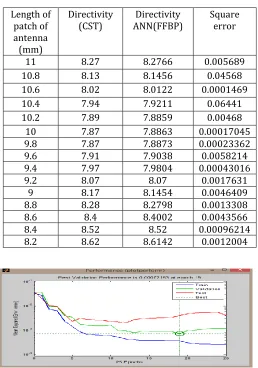
Table.2. Comparison of directivity when calculated using CST software and FFBP ANN

Length of patch of antenna

(mm)

Directivity

(CST) ANN(FFBP) Directivity Square error

11 8.27 8.2766 0.005689

10.8 8.13 8.1456 0.04568

10.6 8.02 8.0122 0.0001469

10.4 7.94 7.9211 0.06441

10.2 7.89 7.8859 0.00468

10 7.87 7.8863 0.00017045

9.8 7.87 7.8873 0.00023362

9.6 7.91 7.9038 0.0058214

9.4 7.97 7.9804 0.00043016

9.2 8.07 8.07 0.0017631

9 8.17 8.1454 0.0046409

8.8 8.28 8.2798 0.0013308

8.6 8.4 8.4002 0.0043566

8.4 8.52 8.52 0.00096214

© 2016, IRJET | Impact Factor value: 4.45 | ISO 9001:2008 Certified Journal | Page 1453 Figure.6: Graph showing the training performance of

directivity and number of epochs to achieve minimum mean square error level in case of FFBP ANN with LM as training algorithm.

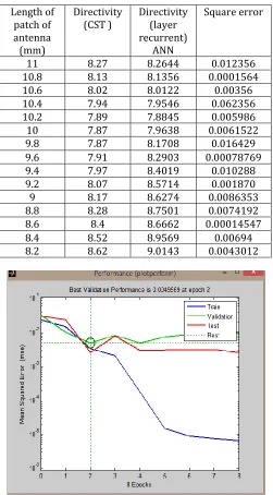
Table 3. Comparison of directivity calculated using CST software and Layer Recurrent ANN

Length of patch of antenna

(mm)

Directivity

(CST ) Directivity (layer recurrent)

ANN

Square error

11 8.27 8.2644 0.012356

10.8 8.13 8.1356 0.0001564

10.6 8.02 8.0122 0.00356

10.4 7.94 7.9546 0.062356

10.2 7.89 7.8845 0.005986

10 7.87 7.9638 0.0061522

9.8 7.87 8.1708 0.016429

9.6 7.91 8.2903 0.00078769

9.4 7.97 8.4019 0.010288

9.2 8.07 8.5714 0.001870

9 8.17 8.6274 0.0086353

8.8 8.28 8.7501 0.0074192

8.6 8.4 8.6662 0.00014547

8.4 8.52 8.9569 0.00694

8.2 8.62 9.0143 0.0043012

Figure.7: Graph showing the training performance of directivity and number of epochs to achieve minimum mean square error level in case of Layer recurrent ANN with LM as training algorithm.

V. RADIATION EFFICIENCY

Radiation Efficiency (U) is a measure of the efficiency with which a radio antenna converts the radio frequency power

accepted at its terminals into radiated power. Another model has been proposed for the analysis of radiation efficiency keeping the training algorithm, error goal and learning rate same for Levenberg-Marquardt training algorithm. The training completes in 8 epochs and the training time was 35 sec. to achieve minimum Mean Square Error (MSE).

Table.4. Comparison of Radiation efficiency when calculated using CST software and FFBP ANN

Length of patch of antenna (mm)

Radiation efficiency (CST)

Radiation efficiency ANN(FFBP)

Square error

11 -3.321 -3.3091 0.010867

10.8 -3.364 -3.2889 0.071123

10.6 -3.315 -3.2942 0.074776

10.4 -3.645 -3.3698 0.11699

10.2 -3.621 -3.6948 0.04934

10 -4.162 -3.9834 0.37938

9.8 -4.314 -3.9887 0.50858

9.6 -3.965 -3.843 0.62137

9.4 -3.266 -3.7534 0.023248

9.2 -4.133 -3.7506 0.074395

9 -4.196 -3.7846 0.85374

8.8 -4.310 -3.8014 0.66298

8.6 -3.116 -3.7814 0.33984

8.4 -3.692 -3.6668 0.3789

8.2 -3.548 -3.4656 0.05518

© 2016, IRJET | Impact Factor value: 4.45 | ISO 9001:2008 Certified Journal | Page 1454

Table.5. Comparison of Radiation efficiency when calculated using CST software and Layer recurrent ANN

Length of patch of antenna

(mm)

Radiation efficiency

(CST)

Radiation efficiency ANN(Layer recurrent)

Square error

11 -3.321 -3.2078 0.11221

10.8 -3.364 -3.2932 0.066847

10.6 -3.315 -3.8302 0.21019

10.4 -3.645 -3.929 0.23096

10.2 -3.621 -3.9675 0.34251

10 -4.162 -3.9317 0.67173

9.8 -4.314 -3.8823 0.2477

9.6 -3.965 -3.8215 0.36845

9.4 -3.266 -3.7534 0.55658

9.2 -4.133 -3.6809 0.52089

9 -4.196 -3.6079 0.082135

8.8 -4.310 -3.5319 0.3219

8.6 -3.116 -4.1833 0.13986

8.4 -3.692 -4.5141 0.18385

8.2 -3.548 -3.4520 0.023194

Figure.8: Graph showing the training performance of radiation efficiency and number of epochs to achieve minimum mean square error level in case of Layer recurrent ANN with LM as training algorithm.

IV.CONCLUSION

An effective configuration methodology for double E-shaped microstrip patch antenna for FR4 substrate in view of ANN has been talked about here. In the analysis network, one can acquire parameters (directivity) of antenna by utilizing length of patch of antenna as inputs. The major advantage of ANN model is that, after proper training, a neural network completely bypasses the repeated use of complex iterative processes for the new design presented to it. This ANN model is suitable for Computer Aided Designing applications.

V. References

[1].Haykin, S., Neural Networks --- A Comprehensive Foundation, Second edition, Prentice-Hall Inc., Boston, 1999.

[2].G. A. Deschamps, “Microstrip microwave antennas,” Presented at the Third USAF Symposium on Antennas, 1953.

[3]. Vegni, L.; Toscano, A.; , "Analysis of microstrip antennas using neural networks," Magnetics, IEEE Transactions on , vol.33, no.2, pp.1414-1419, Mar 1997 doi: 10.1109/20.582522

[4].Carpenter, G. and Grossberg, S. (1998) in Adaptive Resonance Theory (ART), The Handbook of Brain Theory and Neural Networks, (ed. M.A. Arbib), MIT Press, Cambridge, MA, (pp. 79–82

[5].A. Patnaik, R. K. Mishra, G. K. Patra, and S. K. Dash, “An Artificial Neural Network Model for Effective Dielectric Constant of

Microstrip Line”, IEEE Transactions on Antennas and Propagation, vol. 45, No. 11, pp. 1697, 2007.

[6]]. C. A. Balanis, “Antenna Theory, Analysis and Design” John Wiley & Sons, New York, 1997

[7]]. B.-K. Ang and B.-K. Chung, "A wideband E-shaped microstrip patch antenna for 5 - 6 GHz wireless communications," Progress In Electromagnetics Research, Vol. 75, 397-407, 2007

[8]. Kumar, G., and K. P. Ray. Broadband Microstrip Antennas. Boston: Artech House, 2003

.

[9]. Sumit Goyal and Gyandera Kumar Goyal (2011) Cascade and Feedforward Backpropagation Artificial Neural Network Models For Prediction of Sensory Quality of Instant Coffee Flavoured Sterilized Drink. Canadian Journal on Artificial Intelligence, Machine Learning and Pattern Recognition Vol. 2, No. 6, August 2011

[10]. H.Demuth, M. Beale and M.Hagan. “Neural Network Toolbox User‟s Guide”. The MathWorks, Inc., Natrick, USA. 2009.

[11].Grossberg, S. (1976) Adaptive Pattern Classification and Universal ,Recoding: Parallel Development and Coding of Neural Feature Detectors. Biological Cybernetics, 23, 121–134.

[12].Hebb, D.O. (1949) The Organization of Behavior, John Wiley, New York

.

[13].Kohonen, T. (1988) Self-Organization and Associative Memory, Springer-Verlag, New York.

[14].Macready, W.G. and Wolpert, D.H. (1997) The No Free Lunch Theorems. IEEE Transactions on Evolutionary Computing,

1(1), 67–82.

[15].Mandic, D. and Chambers, J. (2001) Recurrent Neural Networks for Prediction: Learning Algorithms, Architectures and Stability, John Wiley & Sons, New York.