Abstract—This paper investigates the possibility of presenting the solution of a discrete-time stochastic control problem in the form of optimal decision regions in the state-time coordinates. We study a problem of optimal management of a mineral extraction project under commodity price uncertainty, with opportunity to switch between several operating modes at the specified decision dates. We use the least-squares Monte Carlo approach and the heuristic Genetic Algorithm to determine the optimal strategies and the time dependent decision boundaries. We investigate the possibility of using the decision boundaries as approximate decision rules for practical applications.
Index Terms—least-squares Monte Carlo, stochastic dynamic programming, time dependent decision rules, real options
I. INTRODUCTION
hile the Discounted Cash Flow or Net Present Value remain the traditional methods of investment valuation in the minerals industry, it has been demonstrated in the literature that failure to address market uncertainty and managerial flexibility in these valuation methods may lead to wrong decisions. Real Options Analysis (ROA) can deal efficiently with the flexibility to revise decisions in response to the evolution of uncertainty and can significantly increase the project value.
The first application of Real Options Analysis to evaluation of a natural resource investment project was introduced by Brennan and Schwartz [1]. They studied the flexibility to delay, temporarily cease or completely abandon the copper mine depending on the stochastic behavior of copper price, and showed that flexible management of the mine can significantly increase the project value. Flexible project management remains an important problem in the valuation of the natural resources investments and has been studied in a number of applications (see, e.g., [2]-[6]).
The least-squares Monte Carlo (LSM) approach, first suggested for pricing of American options by Longstaff and Schwartz [7], is becoming increasingly popular in natural resource investment problems (see, e.g., [4]-[6], [8], [9]).
Manuscript received March 15, 2014; revised April 7, 2014.
Mohammad Mortazavi-Naeini is with the CSIRO Computational Informatics, Minerals Down Under National Research Flagship, North Ryde, NSW, Australia (e-mail: [email protected]).
Tanya Tarnopolskaya is with the CSIRO Computational Informatics, Minerals Down Under National Research Flagship, North Ryde, NSW, Australia (phone: +61 2 9325 3254; e-mail: [email protected]).
Chenming Bao is with the CSIRO Computational Informatics, Clayton,
The valuation of a copper mine originally studied in [1] has been later studied using LSM in [3], [4] and [6]. It has been shown that the problem can be efficiently solved using LSM for multi-factor stochastic models of commodity prices and for extraction of several metals.
A complexity of the real options and stochastic dynamic programming algorithms is arguably among the reasons that such approaches are still rarely used by industry. One of the difficulties of the decision making under uncertainty is that the optimal decisions need to be made in response to evolution of uncertainty. Determining the boundaries of the regions of optimal decisions has been a focus in a number of applications in both deterministic and stochastic continuous optimal control problems (see, e.g., [10]-[13]). Such boundaries are called critical (or threshold) curves, or ‘dispersal curves’ in the aviation applications, and are characterized by non-uniqueness of the optimal strategies at the boundary points. The regions of optimal decisions, also known as decision rules (a mapping of the state space onto the optimal decision space), present the subject that has attracted considerable interest (see e.g, [14], [15]). The evolution of the decision boundaries with time (which can be seen as time dependent decision rules) is an important information that can help industry with understanding and utilizing the results of the analysis.
The focus of this paper is on constructing the decision boundaries for natural resource investment problems. Simulation-based methods for solution of stochastic optimal control problems offer an opportunity to extract the time dependent decision boundaries from the numerical solutions. In this paper, we use the least-squares Monte Carlo approach to get an insight into the structure of the decision regions for a problem of natural resource investment with switching costs. We then use the evolutionary Genetic Algorithm to determine the decision boundaries. We study the behaviour of the decision boundaries with changes in the parameters of the stochastic model of commodity price. Finally, we explore the possibility of using the decision boundaries as approximate time dependent decision rules for practical applications.
II. THE MODEL
We study the natural resource investment problem from the benchmark paper by Brennan and Schwartz [1]. This problems has also been recently studied using the least-squares Monte Carlo approach in [3], [4], [6].
In this example, the management has the option to revise the mine status at pre-determined decision times. The available options are:
close (cease) the mine temporarily. In this case a
Decision Regions for Natural Resource
Investment under Uncertainty
Mohammad Mortazavi-Naeini, Tanya Tarnopolskaya, and Chenming Bao
maintenance cost will be paid. We denote such option by ‘c’;
reopen the temporarily closed mine, by paying the reopening cost. We denote this option by ‘o’; abandon the mine at no cost (‘a’).
At each time step, the mine can be in one of the three modes: operating (o), temporarily ceased (c) and abandoned (a). It is assumed that an abandoned mine cannot be re-opened anymore.
We assume, as in [1], [6], [9], that copper price follows the continuous stochastic process
( ) S
dS r SdtSdZ , (1)
where is the instantaneous standard deviation of the spot price, r is the risk-free interest rate, is the convenience yield, dZSis the increment of a standard Brownian motion.
We consider the time horizon T and assume that a decision to switch between the available options can be made on fixed dates 0t1t2 ...tN T. A constant
inventory level Q and a constant output rate q are assumed for simplicity, as in [1]. The change in the inventory when the project is in operating mode is given by
dQ qdt. (2)
The cashflow at time step
t
nis given by
for , for
0
, ,
for
n n n
n n n
t t t m
n t t t
q S A T S u o
t S M c
a
Q u u
u
(3)
where n
t
S is the copper price, n
t
A
is the operating cost, nt T
is the total income tax and royalties, n
t
M is after-tax maintenance cost. The latter three are given by
0
1 2 1
0
,
( ) max[ ( (1 ) ,0],
, n
n n n n
n
n t t
t t t t
n t t
A A e
T S qS q S A
M M e
(4)
where
is the inflation rate,
1,
2are the royalty rate and the income tax respectively. Switching cost, when changing between options ‘o’ and ‘c’, is given by0
n
n t t
K K e . (5) The objective is to maximize the expected discounted cash
flow over the planning horizon.
III. STRUCTURE OF THE DECISION REGIONS WITH SWITCHING COSTS
In this section, we use the least-squares Monte Carlo approach to solve the problem described in Section II, to determine optimal strategies that maximize the expected discounted cash flow over the planning horizon. The details of the implementation of LSM are given in the Appendix A. The data used in the study are from Brennan and Schwartz and given in the Appendix B.
The accuracy of LSM in application to this problem has been thoroughly tested previously in [3], [4], [6]. In this paper, we use the setting of LSM that was found to produce sufficiently accurate result. The focus of this study is on determining the critical copper prices that trigger changes in the optimal decisions, as functions of time.
The simulation-based LSM method is suitable to get an insight into the optimal decision regions through a mapping of the Monte Carlo realisations for copper prices onto the optimal decision space, for different decision times. Note that for a discrete time stochastic control problem such mapping does not guarantee to produce regions that are clearly separated.
First, we study a simplified version of the problem (1)-(5) with the switching costs set to zero ( 0
n
t
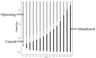
K ). In Fig. 1, each realisation of the copper price for each decision time from 100000 Monte Carlo scenarios and 15 time steps is mapped onto the set of 3 possible decisions (operate, temporarily cease or abandon the mine) which are shown by different colours. In the example shown in Fig. 1, we observe a clear separation of the three regions of optimal decisions. Such clear separation cannot always be obtained from LSM results. We found that in some cases the increase in the number of basis functions and the Monte Carlo sample size may help to improve the separation, but a clear boundary between the decision regions is not generally expected from the solution of a discrete time stochastic control problem.
[image:2.595.334.538.476.599.2]One can see from Fig. 1 that the three regions of optimal decisions undergo transformation with time. The region where it is optimal to temporarily cease the mining operations shrinks as the time goes on and completely disappears before the end of the time horizon, while the region where it is optimal to abandon the mine expands as the end of planning horizon approaches. Such shapes of the decision regions for a finite time horizon problems are intuitively understandable, as one expects that paying maintenance cost to keep the mine temporarily ceased becomes less attractive at the end of the planning horizon. Extensive numerical study shows that the curvature of the decision boundaries increases with increase in the inflation rate.
Fig. 1. Regions of optimal decisions (a mapping of the Monte Carlo realizations of copper price onto the decision space at each time step): ‘operating’ (top, dark grey), ‘ceased’ (intermediate, light grey) and ‘abandoned’ (bottom, black). The model without switching costs; initial price is 0.7, initial decision is ‘operating’.
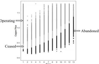
When switching costs are included in the model, the decisions at each decision time become dependent on the decisions at the previous decision time. Figs. 2 and 3 show the mapping of the realisations of the copper price onto the optimal decision space using different shades of grey for different optimal decisions. Figure 2 shows the decision regions for the case when the solution at the previous decision time is to operate the mine, while Fig. 3 shows the regions for the case when the operation was ceased at the previous decision time. We can see that, while the shapes of
Operating
Ceased
the decision regions are similar, the boundaries are in fact different for the two cases.
[image:3.595.76.281.150.280.2]Extensive numerical study shows that compact regions, as those in Figs. 1-3, often cannot be produced using the least-squares Monte Carlo approach. In the following section, we explore the possibility of determining the decision boundaries based on heuristic evolutionary Genetic Algorithm.
Fig. 2. Regions of optimal decisions: ‘operating’ (top, dark grey), ‘ceased’ (intermediate, light grey) and ‘abandoned’ (bottom, black); initial copper price is 0.7, initial decision is ‘operating’; the model with switching costs, the decisions are conditional on u= ‘o’ at the previous decision time.
Fig. 3. Regions of optimal decisions: ‘operating’ (top, dark grey), ‘ceased’ (intermediate, light grey) and ‘abandoned’ (bottom, black). The model with switching costs; initial price is 0.7, initial decision is ‘operating’; the model with switching costs, the decisions are conditional on u= ‘c’ at the previous decision time.
IV. ALGORITHMS TO DETERMINE THE DECISION BOUNDARIES
Figures 1-3 suggest the existence of three regions of optimal decisions and four boundaries, in copper price-time coordinate system, for a problem with switching costs. In what follows, we assume such structure of the solution. We allow for the possibility that the intermediate region (where it is optimal to temporarily cease the mine) may disappear at some time during the time horizon, as shown in Figs. 1-3, and that the lower boundary (between the ‘ceased’ and ‘abandoned’ regions) may become zero. Thus we assume the existence of the four boundary values
1o( ), 2o( ), 1c( ), 2c( )
B t B t B t B t at each decision time t:
1 2 1 2
1 2 1 2
( ), ( ) : 0 ( ) ( ), ( ), ( ) : 0 ( ) ( ).
o o o o
c c c c
B t B t B t B t
B t B t B t B t
(6)
We found that in many cases it is possible to recover such boundaries from the least-squares Monte Carlo approach. To check such possibility, for each decision time we sort the sample of Monte Carlo realizations of copper price into the
(operating, ceased and abandoned) for the two modes (operating or ceased) at the previous decision time. We denote by maxao ( ), maxac ( )
n n
t t
a
a
the maximum values of thesamples corresponding to a decision ‘abandon’ at time step
n
t for optimal decision ‘operate’ and ‘close’ at time step
1
n
t respectively. We denote by min( ), min( )
co cc
n n
t t
a
a
theminimum values and by maxco ( ), maxcc ( )
n n
t t
a
a
the maximumvalues of the samples corresponding to a decision ‘cease’ at time step tn for optimal decision ‘operate’ and ‘cease’ at time step tn1 respectively. Finally, we denote by
min( ), min( )
oo oc
n n
t t
a
a
the minimum values of the samplescorresponding to a decision ‘operate’ at time step tn for optimal decision ‘operate’ and ‘cease’ at time step tn1 respectively. We use LSM solution to establish the decision boundaries if the following conditions are satisfied:
max min max min
max min max min
min max min max
min max min max
( ) ( ), ( ) ( ),
( ) ( ), ( ) ( ),
( ) ( ) , ( ) ( ) ,
( ) ( ) , ( ) ( ) ,
ao co ac cc
n n n n
co oo cc oc
n n n n
co ao cc ac
n n n n
oo co oc cc
n n n n
t t t t
t t t t
t t t t
t t t t
a a a a
a a a a
a a a a
a a a a
(7)
where
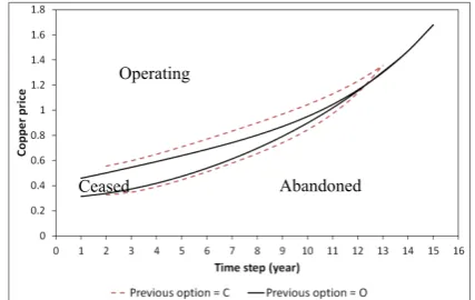
is the tolerance parameter.The decision boundaries that correspond to Figure 1 are shown in Fig. 4, while the decision boundaries that correspond to the solutions shown in Figs. 2 and 3 are shown in Fig. 5.
If the solution satisfying (7) cannot be produced with a reasonable number of Monte Carlo simulations and basis functions, we use Genetic Algorithm to produce the decision boundaries. When Genetic Algorithm is used to produce the decision boundaries, the four values
1o( ), 2o( ), 1c( ), 2c( )
n n n n
B t B t B t B t at each decision time tn,
that satisfy the rules in (6), are treated as unknowns. In this case, we use the partial boundaries produced by LSM to set up the range for GA search. The Genetic Algorithm starts with the random initial population of chromosomes, consisting of genes representing a decision. In this study, each gene represents a value to switch from one option to another. In absence of switching cost there are only two possible genes namely a value to switch between option c and a, and another value to switch between option ‘c’ and ‘o’. However, in presence of switching cost, the current decision is dependent on previous option thus there are two pair of possible options which each of them correspond to the previous option, o or c. The total number of genes in each chromosome is determined by the multiplication of number of years in the planning horizon by number of possible genes in each year. Tournament selection, one-point crossover and bit-wise mutation are used in this study based on the code published at the Kanpur Genetic
Algorithms Laboratory website (http://www.iitk.ac.in/kangal/codes.shtml). Other associated
parameters of GA are set as: number of bits =100, pc=0.99, pm=0.01, population size=500, number of generations= 1000, number of runs=3, tournament size=30 and the Abandoned
Abandoned
Operating Operating
[image:3.595.74.282.332.467.2]Fig. 4. Optimal decision boundaries based on the results presented in Fig 1; the model without switching costs; the initial price is 0.7, the initial decision is ‘operating’.
Fig. 5. Optimal decision boundaries with switching costs, based on the results presented in Figs. 2 and 3. Decision boundaries are shown with solid curves when the optimal decision at the previous decision time is ‘operating’, and with dashed curves when the previous decision is ‘ceased’.
algorithm terminates if there is no improvement in the results after 100 iterations.
We found that the decision boundaries produced by GA are typically non-smooth (see Fig. 6). To rectify this, we smooth the boundaries produced by GA by interpolation, using the polynomial curve fitting. The results are presented in the following section.
V. VALIDATION OF THE DECISION RULES
We found that in many cases the results of LSM analysis satisfy (7) and can be used to produce decision boundaries. If this is not the case, we use GA-based algorithm as described in the previous section.
Figure 6 shows the decision boundaries produced by GA for the initial copper price 0.9. A non-smoothness of the boundaries is clearly observed. Figure 7 shows the boundaries produced by interpolation of the results in Fig. 6, using polynomial functions.
Table I shows a comparison of the project values obtained from LSM and by using the GA-based decision boundaries as decision rules. One can see that using the boundaries produced by GA as decision rules gives an improved project value (expected discounted cash flow), that deteriorates slightly after smoothing.
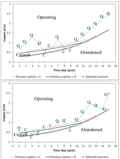
[image:4.595.69.279.220.352.2]Figure 8 illustrates how the decision rules can be used in practice to determine the optimal strategies over the time horizon. For the two cases presented in Fig. 8, the project value computed using the decision rules was identical with the project value computed via LSM. We found that the difference in the project values usually occurs when the copper price at some decision time is close to the decision boundaries.
Fig. 6. Decision boundaries produced by GA-based algorithm for the initial copper price 0.8; the initial decision is ‘operating’. Decision boundaries are shown with solid curves when the optimal decision at the previous decision time is ‘operating’, and with dashed curves when the previous decision is ‘ceased’.
Fig. 7. Decision boundaries produced by interpolation of the decision boundaries obtained via GA-based algorithm for the initial copper price 0.8; the initial option is ‘operating’. Decision boundaries are shown with solid curves when the optimal decision at the previous decision time is ‘operating’, and with dashed curves when the previous decision is ‘ceased’.
The largest difference we observed occurs when the copper price is just below the boundary between the ‘ceased’ and ‘abandoned’ decision regions. The reason is that this is the boundary of an irreversible decision (abandon). We recommend that the decisions near this boundary should be carefully validated using a more rigorous analysis.
For the problem at hand, one would expect the dependence of the decisions on the current state of the inventory. However, we did not observe such dependence, even when we extended the time horizon and reduced the total amount of inventory. An example of the decision boundaries for different states of inventories are shown in Fig. 9. We can see that they all fall on the same curve which coincides with the decision boundary produced without accounting for different states of inventory.
TABLEI
COMPARISON OF PROJECT VALUES,SCALED WITH RESPECT TO LSM VALUES
Copper price
DR(GA) DR (smoothed GA)
0.8 1.000368 0.999393
0.9 1.000106 1.000017
1.0 1.000210 1.000107
VI. PARAMETRIC STUDY
In this section, we study the behavior of the decision boundaries with changes in the parameters of the stochastic copper price model (1).
Operating
Ceased
Abandoned
Operating
Abandoned Ceased
Operating
Ceased Abandoned
Abandoned Ceased
[image:4.595.319.533.243.378.2]Fig. 8. Illustration of the use of decision rules to establish the optimal strategy for two Monte Carlo scenarios of copper price for the initial copper price 0.7 and the initial option ‘operating’ (Scenarios are shown with dotted lines). Dashed curves show the decision boundaries for the case when the previous decision is ‘cease’, while solid curves show the decision boundaries for the case when the previous decision is ‘operating’.
[image:5.595.67.271.49.319.2]
Fig. 9. The boundaries between the ‘abandoned’ and ‘ceased’ decision regions for different states of inventory, when the previous decision time option is ‘ceased’, the initial option is ‘operating’, and the initial copper price is 0.7.
Figure 10 shows the changes in the decision boundaries with the change in the volatility (Eq. 1) for the cases when the decision at the previous decision time is ‘operating’ and ‘ceased’. We can see that the boundary between the ‘ceased’ and ‘operating’ decision regions is practically not affected by changes in the volatility. However, the boundary between the ‘ceased’ and ‘abandoned’ decision regions changes with the change in thevolatility.
Figure 11 shows the changes in the decision boundaries with the change in the risk-free interest rate for the cases when the decision at the previous decision time is ‘operating’ and ‘ceased’ respectively. As in Fig. 10, we can see that the boundary between the ‘ceased’ and ‘operating’ regions is practically not affected by changes in the risk-free interest rate, while the boundary between the ‘ceased’ and ‘abandoned’ decision regions changes with the change in the risk-free interest rate.
Fig. 10. Changes in the decision boundaries with changes in the volatility between 5% and 8% for the initial price 0.7 and the initial option is ‘operating’. The previous decision time option is: ‘ceased’ (top), and ‘operating’ (bottom).
Fig. 11. Changes in the decision boundaries with changes in the risk-free interest rate between 6% and 10% for the initial price 0.7 and the initial option is ‘operating’. The previous decision time option is: ‘ceased’ (top) and ‘operating’ (bottom).
VII. CONCLUSIONS
Using the example of mineral extraction project, we showed that the solution of discrete time optimal control problem can be presented in the form of optimal decision regions in the state-time coordinates. An encouraging result is a relative insensitivity of the decision boundaries to changes in the parameters of the stochastic model of commodity price. We found that the boundary between the regions where it is optimal to abandon the mine and where it is optimal to temporarily cease the extraction is the most
Ceased
Abandoned O O
O O
C C
O
C C O
O O O
O O
O C C C
C C O O
C O
O O
O O
O Abandoned
Abandoned Ceased
Operating
Operating
Operating Operating
Abandoned
Abandoned
Abandoned Abandoned
Ceased Ceased Operating
Operating
0.05 0.06 0.07 0.08
0.05 0.06 0.07 0.08
0.06
0.07 0.08 0.09 0.1
0.06 0.07
0.08 0.09 0.1
[image:5.595.325.525.352.610.2] [image:5.595.65.273.388.518.2]sensitive boundary. This is understandable, as this boundary is associated with an irreversible decision. We found that the project value can be significantly affected by inaccuracy in this boundary. We therefore suggest that the decision to abandon the mine needs to be carefully verified if the commodity price is in the vicinity of this decision boundary.
We found that the decision boundaries computed using the Genetic Algorithm are usually non-smooth. To overcome this, we used a polynomial function interpolation to smooth the boundaries. Numerical results show that smoothing the boundaries affects the objective function only marginally, and the expected discounted cash flow may still outperform the one computed using LSM algorithm. A parametric representation of the boundaries for the purpose of GA analysis might be useful and will be the subject of further study. Also, an improved computational efficiency of the Genetic Algorithm will be further investigated.
Despite expectations, we found that the decision rules for this particular problem are independent of the state of inventory. We expect that this is an exception rather than a common rule, and may be a result of a simplified nature of the problem. Dependence on the state of inventory needs to be examined carefully for more complex natural resource investment problems.
We expect that establishing the decision boundaries (decision rules) for high-dimensional stochastic optimal control problems may be too difficult and not practical. Nevertheless, understanding the structure of the decision regions and its sensitivity to changes in the parameters of the stochastic processes is important for practical purposes, as it gives practitioners an insight into the decision under uncertainty process and into the forthcoming optimal decisions, and alerts them to the conditions when the actions may be required.
APPENDIX A:LEAST-SQUARES MONTE CARLO ALGORITHM. Discretised version of the diffusion process in (1) is given by
2
1 exp ( / 2)( 1 ) 1 1 ,
n n n
t t n n n n t
S S r t t t t Z
where 1 (0,1) i.i.d. n
t
Z N
The Bellman value function for the optimal switching problem described in Section 3 is given by
1 1 1 1
( , , , ) max ( , , , ) ( )
[ ( , , , ) , , ] ,
k
k k k o o k
r t
k k k k k k k
o O k k k k
V S Q o t S Q o t K t
e E V S Q o t S Q o
where r is the risk-free interest rate and Ek[.] is the expectation conditional on the information available at time
k
t . We denote by
1 1 1 1
( , , , ) [ ( , , , ) , , ]
r t
k
k k k k k k k k k k
S Q o t e E V S Q o t S Q o the continuation value in Bellman equation and approximate it by a finite set of basis functions
l,
l 0, ...,L
( , , , )
S Q o tk k k k
0
(
,
, ) ( ).
L
l l k k k l k
Q o t S
The coefficients iare found by the least squares fitting in the backward recursion, determining the optimal exercise
policy and revising the remaining cashflow along the path.
APPENDIX B:DATA FOR NUMERICAL STUDY
We used annual decisions and 15 year planning horizon. The number of Monte Carlo simulations in the base case is 100000. In agreement with [6] we found that the Laguerre polynomials produce the best results.
TABLE BI
PARAMETERS FOR VALUATION OF THE INVESTMENT
Output rate (q) 10 million lbs/year
Inventory(Q) 150 million lbs
Initial average production cost(A0) $0.50/lb
Initial cost of opening $200,000 Initial cost of closing $200,000
Initial maintenance cost(M0) $500,000/year
Convenience yield(δ) 1%/year Price volatility (σ) 8%/year Interest rate, nominal (r) 10%/year
Inflation rate (π) 8%/year
Property taxes, operating/closed 2%/year
Income taxes (τ2) 50%/year
Royalty taxes (τ1) 0%/year
REFERENCES
[1] M.J. Brennan, and E.S. Schwartz, “Evaluating natural resource investment”, The Journal of Business, vol. 58, no. 2, pp. 135-157, 1985.
[2] L. Trigeorgis, “Real options: managerial flexibility and strategy in resource allocation”. MIT Press: Cambridge, MA, 1996.
[3] A.E. Tsekrekos, M.B. Shackleton, and R. Wojakowski, “Evaluating natural resource investment under different model dynamics: managerial insights”, European Financial Management, vol. 18, no. 4, pp. 543-577, 2012.
[4] S.A. Abdel Sabour, and R. Poulin, “Valuing real capital investments using the least-squares Mone Carlo method”, Engineering Economist, vol. 51, pp.141-160, 2006.
[5] R.G. Dimitrakopoulos, and S.A. Abdel Sabour, “Evaluating mine plans under uncertainty: Can the real options make a difference?”, Resources Policy, vol. 32, pp. 116-125, 2007.
[6] A. Gamba, “Real options: a Monte Carlo approach”. In Handbooks in Finance: Real Options , G.A. Sick, and S. Myers, Eds, North Holland, 2009.
[7] F. Longstaff, and E. Schwartz, “Valuing American options by simulations: a simple least-squares approach”, Review of Financial Studies, vol. 14, no. 1, pp. 113-147, 2001.
[8] C. Bao, M. Mortazavi-Naeini, S. Northey, T. Tarnopolskaya, A. Monch, A. Zhu, “Valuing flexible operating strategies in nickel production under uncertainty”, in MODSIM2013, 20th International Congress on Modelling and Simulations, 2013, pp. 1426-1432. [9] C. Bao and Z. Zhu, “Land use decisions under uncertainty: optimal
strategies to switch between agriculture and afforestation”, in MODSIM2013, 20th International Congress on Modelling and Simulations, 2013, pp. 1419-1425.
[10] V. Gaitsgory and T. Tarnopolskaya, “On adoption of new technology under uncertainty”, in MODSIM2013, 20th International Congress on Modelling and Simulations, 2013, pp. 1433-1439.
[11] T. Tarnopolskaya, and N. Fulton, “Dispersal curves for optimal collision avoidance in a close proximity encounter: a case of participants with unequal turn rates”, in Proceedings of the World Congress on Engineering 2010 (WCE 2010), pp. 1789-1794.
[12] T. Tarnopolskaya, and N. Fulton, “Non-unique optimal collision avoidance strategies for coplanar encounter of participants with unequal turn capabilities”, IAENG International Journal of Applied Mathematics, vol. 40, no. 4, pp. 289-296, 2010.
[13] T. Tarnopolskaya, and N. Fulton, “Synthesis of optimal control for cooperative collision avoidance for aircraft (ships) with unequal turn capabilities”, Journal of Optimization Theory and Applications, vol. 144, no. 2, pp. 367-390, 2010.
[14] J. Thenie and J.-Ph. Vial, “Step decision rules for multistage stochastic programming: a heuristic approach”, Automatica, vol. 44, no. 6, pp. 1569-1584, 2008.