Abstract—In Access Point(AP) Localization, a lot of manual efforts are required to acquire necessary information of the APs to be localized for precise localization, but little research has been devoted to the problem on how to select appropriate measurement points for lower cost and with high accuracy. This paper presents an approach to optimize the selection of meas-urement points. The idea is that the next measmeas-urement point is determined based on real-time measurement, and it is located at the intersection of the coverage area of APs, whose locations are roughly estimated by the previously measurement information, so as to detect as many APs as possible at each measurement point. Simulation results show that the proposed algorithm can reduce the number of necessary measurement points and im-prove accuracy.
Index Terms—Access Point(AP) localization, measurement point selection, information collection
I. INTRODUCTION
he localization of mobile devices in wireless environ-ments has attracted much attention[1], but they are often estimated with prior knowledge of the location of the access point(AP). When there is limited prior knowledge, for ex-ample, anonymous environment, however, the localizing of access points is required. Besides, AP localization is also important for wireless network management and locating unauthorized APs[2].
Recently, several attempts have been made for access point(AP) localization. Han et al. [3] considered the trend of receive signal strength(RSS) by comparing value of RSS in different measurement points. Koo and Cha [4] considered the relative positions of each AP and calculated real positions of APs later using multidimensional scaling (MDS) tech-niques. Subramanian et al. [5] used directional antenna to estimate the direction of the APs and calculated the position of APs by k-means method. Seung [6] proposed a modified version of the Hata-Okumara model to calculate the distance information inferred from the measured signal strength.
These approaches have a common feature: AP localization includes two phases: first, massive information should be collected at many measurement points, and then a certain localization method is used to estimate the locations of APs. Generally, the first phase is a time-consuming process and requires extensive manual efforts. Typically, several hours or
Manuscript received November 16, 2014.
Xiaoling Yang, Bing Chen and Fengyu Gao are with the Department of Computer Science and Technology, Nanjing University of Aeronautics and Astronautics, P.R. China (corresponding author to provide phone: 0086-15298363068, e-mail: [email protected]; [email protected]; [email protected]).
even more time is required to collect such an amount of data when the area considered is very large. However, the focus in current literatures about AP localization is the localization method, and little research has been devoted to clearly esti-mate how many measurement points are needed and where to measure in a given workspace to improve accuracy and re-duce the measurement costs. This paper considers the prob-lem on how to select suitable measurement points to collect enough information for AP localization, we consider online AP localization, that’s to say, the location of AP is estimated while collecting information. The closest research to our objective is Zhang’s work in [7], they tried to locate an AP by guiding the next measurement point based on the current information, but only one AP is located each time and it is inappropriate for localizing multiple APs.
In this work, we propose an approach that aims at getting a balance between overall accuracy and manual efforts. To reduce manual efforts, there should be as many APs as pos-sible to be detected in each measurement point. We estimate the locations of APs based on previous measurements and select some point at the intersection of the coverage area of the APs as the next measurement point. This approach can ensure the validity of measurement points for AP localization. To the best of our knowledge, there have been no previous attempts to develop a method for the selection of measure-ment points in multiple APs localization. Simulation results show that the proposed algorithm can reduce the number of measurement points and improve localization accuracy.
II.METRIC OF MANUAL EFFORTS IN APLOCALIZATION
To collect enough information, measurements should be taken in many points, the number of which is indicated as
N
P, andl
is the total length of the path from the first point to the last. For each measurement point, an RSS sample (a set of RSS values) is collected. As RSS values vary noticeably due to interference and environment conditions, several consecu-tive RSS measurements need to be collected for each sample. We assumet
S is the time needed to get an RSS sample, andv
is the speed of the worker. The total timet
is formulated as follows:/
P St
N
t
l v
(1) Measurement points should be selected in order to achieve a reasonable coverage of the APs. On one hand, increasing the number of measurement points generally leads to better accuracy; on the other hand, it requires more efforts. However, the effectiveness of a selection pattern highly depends on the detailed workspace conditions, i.e., the number and positionsHow to Select Measurement Points in Access
Point Localization
Xiaoling Yang, Bing Chen, and Fengyu Gao
of APs to be localized. Unfortunately, there is not any related work, especially for multiple APs. Therefore, the objective of this work is to select a reasonable number of measurement points while getting enough accuracy.
III. SELECTION OF MEASUREMENT POINTS
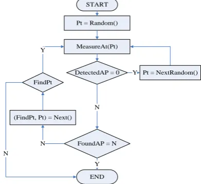
The workflow of the proposed approach is shown in Fig. 1. First, a point is randomly selected as the first measurement point, and the positions of APs are estimated according to the collected measurement information. If there is no AP whose position has been estimated, choose the next point according to the current measurement points (details available in 3.1, NextRandom). Or else, we would check if all the APs are found; if not, we would choose the next point according to either the intersection area or the extended area (details available in 3.2, Next). We keep moving on to the next point until all the APs are found. The functions and variables are explained as follows:
Random(): selects a point randomly;
MeasureAt(Pt): gets the measurement information at point Pt;
DetectedAP: the number of APs whose positions have been estimated;
NextRandom(): randomly generates a point based on the current measurement point and all the previous meas-urement points;
FoundAP: the number of APs which have been found, the total number of APs to be localized is N;
Next(): selects a point at the intersection area of the coverage areas of predicted APs; if there is no available point at the intersection area, select the point at the ex-tended area.
Pt = Random()
MeasureAt(Pt)
DetectedAP = 0 Y
N
FoundAP = N
Y Y
(FindPt, Pt) = Next()
END
Pt = NextRandom() START
N FindPt
[image:2.595.77.273.453.632.2]N
Fig. 1. Workflow of the proposed approach
Some notations in the approach are described as follows: ▪AllMPtList: the list of points where have measured. ▪EstiApLocDict: it is represented by tuple <ApName,
ApLoc>, ApName means the name of AP and ApLoc means the estimated position of the corresponding AP. ▪AllMApInfoNum: It is represented by tuple <ApName,
Number>, ApName means the name of AP, Number means the amount of measurement information of the corresponding AP. It is used to assess the priority of Aps, the less information, the higher the priority of the AP.
▪miniDistance: it is represented by integer, it means the minimum distance between measurement points.
▪ExperimentArea: it means the area of experiment and is represented by a rectangle.
A. Case 1: NextRandom
Given the current measurement point (denoted by tMPt) and the initial extended distance (denoted by ExtendDist), the next measurement point is calculated in detail by Algorithm 1. CalcPtFromPt(…) returns a point according to angle and distance away from an original point. IsFarFromAllMPts(…) represents whether the point is far away from all the previous measurement points; if it is, returns true, or else, returns false.
Algorithm 1: NextRandom()
Require: Point tMPt ≠null {the current measurement point}
Require: Integer ExtendDist ≠ 0 {the distance from TempMPt}
Require: Integer AngleNum ≠ 0 {the number of angles to be calculated in each ExtendDist}
1. {calculate the longest distance that could be extended}
2. Integer MaxDist = max(||tMPt, P1||,…,||tMPt, P4||), where P1…P4 are the four points in ExperimentArea and ||tMPt, P1|| means the distance be-tween tMPt and P1.
3. Integer Num = 0
4. While ExtendDist <= MaxDist do 5. If Num > AngleNum do
6. Num = 0, ExtendDist = ExtendDist + miniDistance 7. Else do
8. Integer angle = Randomly generate an angle in [0, 360) 9. Point Pt = CalcPtFromPt(tMPt, ExtendDist, angle) 10. If IsFarFromAllMPts(Pt) do
11. Return Pt {the next measurement point is found} 12. End If
13. Num = Num + 1 14. End If
15. End While
B. Case 2: Next
Given the current measurement point (denoted by tMPt), the next measurement point is calculated in detail by Algo-rithm 2. Some functions are detailed as follows:
GetPrioSortApList(…): gets an AP list in descending order
of priority according to the amount of information, the less information, the higher the priority of the AP.
CalcInterSection(…): calculates the intersection rectangle
according to the given AP list and their respective estimated locations.
The calculation about intersection rectangle of two APs’ coverage area is shown in Fig. 2.
EAP
1 represents the cov-erage area of AP1, which is denoted by circles determined by their positions and transmit power. The intersection area is denoted byP
1,P
2,P
3 andP
4 as shown in Fig. 2, and they can be calculated easily. Meanwhile, in order to simplify, the intersection area of two APs’ coverage areas is represented by a rectangle approximately, which is represented by a black rectangle in Fig. 2.x
1,x
2,y
1 andy
2 can be calculated by the following formula(2). Thus, the corresponding rectangle is calculated.1
2
1
2
min( 1. , 2. , 3. , 4. )
max( 1. , 2. , 3. , 4. ) min( 1. , 2. , 3. , 4. )
max( 1. , 2. , 3. , 4. )
. .
x P x P x P x P x
x P x P x P x P x y P y P y P y P y
y P y P y P y P y
where Pi x and Pi y mean the value in x axis and y axis
1
EAP
EAP
23
EAP
EAP
4Intersection rectangle Coverage area of an AP
1 2 3 4 5 6 N-1 N
Rectangle 1
…
Rectangle 2 Rectangle 3 Rectangle M
many temporary rectangles
The Final Rectangle
[image:3.595.148.529.41.538.2]Fig. 3. Calculation of intersection rectangle of three APs Fig. 2. Calculation of intersection rectangle of two APs
1
EAP EAP2
3
EAP
Coverage area of an AP Intersection rectangle Of EAP1 and EAP2
Intersection rectangle Of EAP2 and EAP3
Intersection rectangle Of these three AP
2 P 3 P 1 P
4 P
1
EAP
2
EAP
x y
1
x
x
21
y
[image:3.595.299.506.56.195.2]2
y
Fig. 4. Calculation of intersection rectangle of four APs Fig. 5. Calculation of intersection rectangle according to AP list
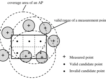
Fig. 6. Example about valid candidate point in intersection area
Measured point Valid candidate point Invalid candidate point The extended area
The intersection area valid area of a measurement point
coverage area of an AP
Measured point
Valid candidate point
Invalid candidate point valid range of a measurement point
Fig. 7. Example about valid candidate point in extended rectangle
The calculation of intersection rectangle of multiple APs is shown in Fig. 3 and Fig. 4, which represents the number of APs is odd and even, respectively.
When calculating the intersection rectangle according to the given AP list, if the number of APs listed is only 1, the intersection rectangle is the bounding rectangle of the cov-erage area of AP. Or else, the intersection rectangle of mul-tiple APs is calculated as shown in Fig. 5, for example, if there are N APs in the list, first, select two APs sequentially and calculate the intersection rectangle of these two APs. If N is odd, the last AP (N) is calculated with the prior AP (N-1). Then, M rectangles are obtained, M = (N-1)/2 + 1. Thus, the intersection rectangle of M rectangles is calculated. Finally, the final intersection rectangle is calculated.
CalcPtByRect(…): calculates the next point according to
the given rectangle. Fig. 6 shows an example. The rectangle box with solid line represents the intersection rectangle of APs. First, the intersection rectangle is divided into many cells according to miniDistance, and the center point of each
cell is chosen as the candidate point, which forms a set of points, indicated by Q, then another set of points, indicated by P, can be calculated by formula (3):
{ | ( ), }
[image:3.595.313.533.371.532.2] [image:3.595.58.238.389.526.2]P pt IsFarFromAllMPts pt ptQ (3) They are the valid points in Fig. 6. If P is empty, this in-dicates that the next measure point cannot be calculated ac-cording to intersection rectangle, or else, the next measure-ment point can be calculated by formula (4):
arg min || , ||,
|| , || tan int
NextMeasurePt tMPt pt pt P
where tMPt pt means the dis ce between these two po s
(4)
Group(…): calculates the combinations that choose a given
number APs from a given AP list. For example, if the AP list is {0, 1, 2, 3} and number is 3, all the combinations in order are as below: { {0, 1, 2}, {0, 1, 3}, {0, 2, 3}, {1, 2, 3} }.
GetRectByAp(…): given a point and distance, obtains the
CalcPtFromExtendRect(…):given a rectangle, the next
point is calculated by extending each side a miniDistance each time. Fig. 7 shows an example. All the valid candidate points form a set of points, indicated by P. If P is not empty, the point nearest the current measurement point from P is chosen as the next measurement point. Or else, this indicates that the next measurement point cannot be found.
Algorithm 2: Next()
Require: Point tMPt ≠null {the current measurement point} 1. {get the sorted AP list}
2. thisSortedApList = GetPrioSortApList(AllMApInfoNum) 3. Integer ApNum = Count(EstiAPLocDict)
4. ApList = null {the AP list to be calculated}
5. Rectangle Rect = null {the intersection rectangle calculated according to ApList}
6. Point Pt = null {the temporary point} 7. While ApNum > 0
8. If Count(AllMApInfoNum) = 0
9. {there is no information to assess the priority of APs} 10. ApList = choose ApNum APs from EstiApLocDict in order 11. If CalcInterSection(ApList) and Pt = CalcPtByRect(Rect) 12. FindPt = true, Return Pt { find the next measurement point } 13. Else do
14. ApNum – 1 15. End If
16. Else
17. { get all the combinations in order in thisSortedApList } 18. For ApList in Group(thisSortedApList, ApNum)
19. If CalcInterSection(ApList) and Pt = CalcPtByRect(Rect) 20. FindPt = true, Return Pt {find the next measurement point} 21. End If
22. End For 23. ApNum – 1 24. End If
25. End While
26. {there is no next measurement point in the intersection area, the ex-tended area would be calculated}
27. {Get the estimated location of the AP which has the highest priority} 28. Point ApLoc = GetHighestPrioApLoc()
29. {Get the rounding rectangle of the coverage area of the AP who has the highest priority}
30. Rectangle OriginRect = GetRectByAp(ApLoc) 31. While OriginRect < ExperimentArea
32. If Pt = CalcPtFromExtendRect(OriginRect)
33. FindPt = true, Return Pt {find the next measurement point } 34. End If
35. End While
36. {there is no next measurement point in the ExperimentArea} 37. FindPt = false
IV. EXPERIMENT
A. Simulation Platform and Configuration
We evaluated the performance of the proposed approach with our own simulation platform. DriveByLoc[5] is chosen as the AP localization method, which records the directions of APs in each measurement point with a directional antenna and uses k-means algorithm to estimate the locations of APs. We simulate the directional antenna and measure information per 30 degrees.
The APs to be localized are put randomly in the experiment area. Since the effectiveness of a selection pattern about measurement points highly depends on the detailed work-space conditions, i.e., the number and positions of APs to be localized, thus, we vary the number and positions of APs. The number of APs is 1, 5, 10 and 20. Five AP layouts are ran-domly generated under each setting, and each experiment is repeated ten times. Since the transmit power of each AP may be different, we varied
P
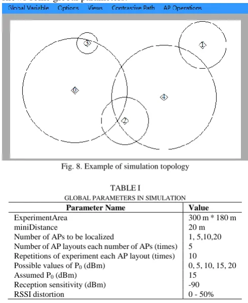
0 from 0 to 20 dBm. Andconsid-ering the real wireless communication environment between the AP and receiver, we varied RSS distortion, which is af-fected by shadow fading, multi-path and small fading effects. Fig. 8 shows an example of simulation topology. Table I shows some global parameters.
Fig. 8. Example of simulation topology
TABLEI
GLOBAL PARAMETERS IN SIMULATION
Parameter Name Value
ExperimentArea 300 m * 180 m
miniDistance 20 m
Number of APs to be localized 1, 5,10,20
Number of AP layouts each number of APs (times) 5 Repetitions of experiment each AP layout (times) 10
Possible values of P0 (dBm) 0, 5, 10, 15, 20
Assumed P0 (dBm) 15
Reception sensitivity (dBm) -90
RSSI distortion 0 - 50%
B. Simulation Results
In this section, we evaluate the performance of the pro-posed algorithm. Since most approaches about AP localiza-tion have not considered neither multiple APs localizalocaliza-tion nor the selection of measurement points, the proposed approach cannot be compared with existing methods. We compare InterArea we proposed with Random. In Random, like the case 1 (NextRandom), the next measurement point is calcu-lated by randomly selecting an angle from the current meas-urement point.
As for the manual efforts in formula 1,
t
s is related to three factors: the number of measurement angles, the repetition of each measurement and the time taken in each measurement. The number of measurement angles is 12, the repetition of each measurement is 10 and the time taken in each meas-urement is almost 1 second, thust
s is almost 120.v
is the same with whether InterArea or Random, and the value is set to be 1 m/s.l
is related toN
p and the locations of meas-urement points. [image:4.595.303.548.109.409.2]Fig. 9. Manual efforts with InterArea and Random Fig. 10. CDF of error distance with RSS distortion 0 - 10%
[image:5.595.53.272.274.451.2]Fig. 11. CDF of error distance with RSS distortion 0 - 20% Fig. 12. CDF of error distance with RSS distortion 0 - 50%
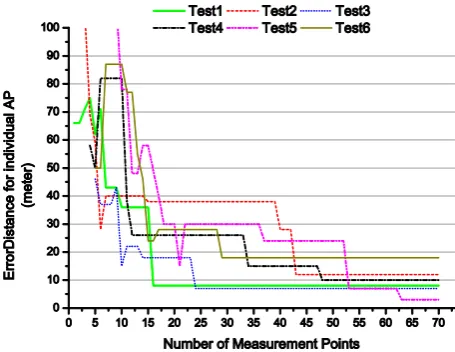
Fig. 13. Relationship between measurement point and error distance of indi-vidual AP when only one AP need be localized
Fig. 14. Relationship between measurement point and error distance of individual AP when more than one APs need to be localized
Next, we consider the effect of the number of measurement points and the RSS distortion on the Cumulative Distribution Function (CDF) of error distance, as shown in Fig. 10 - 12, wherein, 70-InterArea means that it is the result with a total of 70 measurement points and the next measurement point is calculated with InterArea.
Fig. 10 shows the CDF of error distance when the RSS distortion ranges from 0 to 10% and the number of
[image:5.595.311.534.276.453.2] [image:5.595.313.541.480.656.2] [image:5.595.55.279.481.655.2]m with Random. And in case of 30 measurement points, the accuracy (with probability of 90%) is 25 m with InterArea and 40 m with Random.
To prove our proposed algorithm, we change the distortion to 0 to 20%, as shown in Fig. 11. When there is a total of 70 measurement points, the localization accuracy (with proba-bility of 90%) is 15 m with InterArea and 30 m with Random. When the total number is down to 50, the accuracy (with probability of 90%) is about 20 m with InterArea, but is re-duced to about 40 m with Random. In case of 30 measurement points, the accuracy (with probability of 90%) is 30 m with InterArea and more than 50 m with Random.
Further, we change the distortion to 0 to 50%, the result is shown in Fig. 12. It can be seen that, the accuracy (with probability of 90%) reduces to 25 m with InterArea and about 55 m with Random in case of a total of 70 measurement points. And the fewer the total of measurement points, the lower the accuracy.
It can be shown that, the accuracy with InterArea is higher than with Random.
Next, we analyze the relationship between the individual AP localization error distance and the number of measure-ment points, as shown in Fig. 13 and Fig. 14, where, Fig. 13 shows the relationship in case of only one AP to be localized, and Fig. 14 shows the relationship when there are many AP to be localized. To facilitate a clear expression, six tests are chosen from ten tests in the simulation. It can be seen that the change of error for individual AP may be divided into three stages: first, the error distance may change slowly or jitter, then gradually decreases, and finally reaches a smooth min-imum value. In the second stage, the error distance gradually decreases, but it may remain unchanged in certain period, which may be longer when there are many APs to be localized, as can be seen from the comparison of Fig. 13 and Fig. 14. The reason is that when there are many APs to be localized, the location of the next measurement point is determined according to the priority of APs; the higher the priority of AP, the more likely the next measurement point is biased toward the AP, which may lead to a lower possibility of detecting other APs in the next measurement point, and the error of other APs may remain unchanged. However, if there is only one AP to be localized, all the measurement points are cal-culated for estimating the location of this AP, resulting in a shorter period. Thus, the more the APs to be localized, the longer the error remains unchanged for an individual AP.
V.CONCLUSION
Most approaches about AP localization focus on the lo-calization method and the selection of measurement points attracts little attention, however, in fact, the number and cations of measurement points are closely related to the lo-calization accuracy. In this paper, we have proposed a new method for optimizing the selection of measurement points in AP localization. The main idea is that, the next measurement point is determined by the intersection of the coverage area of APs, whose locations are roughly estimated by the previously measured information, so that as many APs as possible are detected at each measurement point. To do this, we divide the selection of the next measurement point into two cases: the
point is calculated according to the current measurement point, or based on the intersection or extending area of coverage area of APs. Simulation results show that AP localization with InterArea we have proposed, compared with Random, en-sures the validity of measurement points for localization and reduces the total number of the measurement points and im-proves localization accuracy. And it is adequate both for single and multiple AP localization.
While this approach so far is evaluated by simulation, it can be extended to the actual environment, then an environment map should be imported into the system and the detailed environment should be considered when calculating the next measurement point. We will consider this in the future. We expect that better localization would be got with the proposed approach.
ACKNOWLEDGMENT
The authors thank the reviewers for their comments which helped improve the paper.
REFERENCES
[1] A. Kushki, K.N. Plataniotis, and A.N. Venetsanopoulos, “Intelligent dynamic radio tracking in indoor wireless local area networks,” Mobile Computing, IEEE Transactions on, 2010, 9(3): 405-419.
[2] T.M. Le, R.P. Liu, and M. Hedley, “Rogue access point detection and localization,” Personal Indoor and Mobile Radio Communications (PIMRC), 2012 IEEE 23rd International Symposium on. IEEE, 2012: 2489-2493.
[3] D. Han, D.G. Andersen, M. Kaminsky, K. Papagiannaki, S. Seshan,
“Access point localization using local signal strength gradient,” Passive and Active Network Measurement. Springer Berlin Heidelberg, 2009: 99-108.
[4] J. Koo and H. Cha, “Unsupervised Locating of wifi access points using smartphones,” Systems, Man, and Cybernetics, Part C: Applications and Reviews, IEEE Transactions on, 2012, 42(6): 1341-1353.
[5] A.P. Subramanian, P. Deshpande, J. Gaojgao J, and S.R. Das, “Drive-by localization of roadside WiFi networks,” INFOCOM 2008. The 27th Conference on Computer Communications. IEEE, 2008.
[6] S. Nam, “Localization of access points based on signal strength meas-ured by a mobile user node,” IEEE Communications letters. 18(8). 2014.