Genetic Algorithm based Modification of Production Schedule for Variance Minimisation of Energy Consumption

Genetic Algorithm based Modification of

Production Schedule for Variance Minimisation of

Energy Consumption

C. Duerden, L.-K. Shark, G. Hall, J. Howe

Abstract – Typical manufacturing scheduling algorithms do not consider the energy consumption of each job, or its variance, when they generate a production schedule. This can become problematic for manufacturers when local infrastructure has limited energy distribution capabilities. In this paper, a genetic algorithm based schedule modification algorithm is presented. By referencing energy consumption models for each job, adjustments are made to the original schedule so that it produces a minimal variance in the total energy consumption in a multi-process manufacturing production line, all while operating within the constraints of the manufacturing line and individual processes. Empirical results show a significant reduction in energy consumption variance can be achieved on schedules containing multiple concurrent jobs.

Index terms – Energy consumption optimisation, Genetic algorithms, Peak energy, Schedule optimisation

I. INTRODUCTION

_{Scheduling manufacturing jobs and ensuring that they}

operate within the capabilities of the manufacturing production line is fundamental in mass production and high volume manufacturing. The goal of a traditional scheduling algorithm [1] is to allocate limited machinery and equipment to manufacturing jobs without taking into account how this will affect the energy consumption at the production line level, and how it will vary as the schedule is being executed. This can potentially limit the availability of a manufacturing production line as the infrastructure can only deliver a certain amount of energy at any given time. Ideally, for manufacturers an optimal schedule is one which completes all required jobs in the least amount of time and consumes the minimal amount of energy at any given instance, thus increasing the productivity and availability of the production line while reducing costs. However this is hindered by many scheduling problems being NP-hard and therefore cannot be

Manuscript received June 30th _{2014; revised July 25}th _{2014. This work is}

financially supported by BAE Systems (Operations) Ltd and the Engineering and Physical Sciences Research Council (EPSRC) as part of a CASE studentship.

C. Duerden and G. Hall are with the Advanced Digital Manufacturing Research Centre, University of Central Lancashire, Burnley Campus, Burnley, Lancashire, BB12 0EQ, UK (phone: 01772 896093; email: [email protected], [email protected]).

L.-K.Shark is head of the Advanced Digital Manufacturing Research Centre, University of Central Lancashire, Preston Campus, Preston,

Lancashire, PR1 2HE, UK (phone: 01772 893253; email:

[email protected]).

J. Howe is head of the Centre for Energy and Power Management, University of Central Lancashire, Preston Campus, Preston, Lancashire, PR1 2HE, UK (phone: 01772 894220; email: [email protected]).

practically optimised by schedulers that are based on polynomial-time algorithms. Despite this, work has been undertaken to include additional objectives for traditional schedulers to work towards. Fang et al and Pechmann et al both present methodologies for production schedules which aim to also minimise peak energy consumption [2]-[4]. As does the commercial scheduling software E-PPS by Transfact [5]. While the work of Fang et al and Pechmann et al shows promising results, it is concluded by Fang et al that finding the optimal schedule is difficult due to the complexity of the problem and its NP-hard nature. Electrical energy is undoubtedly one of the most valuable resources available to manufacturers. In 2012 UK industry consumed approximately 97.82 TWh (8411 ktoe) [6]. Recently there have been numerous works on intelligent scheduling which aims to reduce manufacturing energy consumption by reducing the idling times of and by putting the machine into energy saving modes or shut them down entirely [7]-[9]. The main purpose of the latter is to ensure the machine is ready to run when the next job arrives. In their proposed systems, by intelligently deciding when to shut down a machine or put it into an energy saving mode, the total energy consumption for the production line can be reduced. While all these show promising results, the problem with generating energy optimised schedules has received little attention and appears to be plagued by its NP-hard nature. The use of artificial intelligence in the generation of manufacturing schedules has shown some promising results. Genetic algorithms appear to be a popular choice for solving scheduling optimisation which can include multi-objective [10], [11] and multi-project [12] problems.

Although there have been investigations into multi-objective scheduling algorithms which produce a valid schedule while aiming to reduce the peak, or variance in the energy consumption [10], the optimal solution is difficult to find when using traditional methods and algorithms due to a very large search space. While artificial intelligence has been shown to be capable of solving schedule optimisation problems in an efficient manner [10]-[12], it is noted that the schedule optimisation systems are designed to perform the entire scheduling process. This may present manufactures with a disadvantage if a set of jobs needs to be completed as quickly as possible with no concern for energy consumption. An example of which is a product order with a short lead time. To the authors knowledge it is unknown how well these systems can be adjusted to produce a schedule suited to the manufacturers changing preferences.

schedule produced by a traditional scheduling algorithm, in order to minimise the variance in production line energy consumption without exceeding the overall production deadline. The technique used is inspired by load-shifting, a traditional energy optimisation method in which energy intensive jobs are scheduled to run during times of low energy tariffs [13].Following the methodology described in section 2, experiments and results are presented to demonstrate the level of potential reduction in energy consumption variance.

II. METHODOLOGY

In the proposed system, a schedule for a series of manufacturing jobs is initially generated using traditional scheduling algorithms. This takes in a list of jobs to be processed and produces a schedule which ensures that a) all jobs are processed in the correct order; b) the total makespan for each process and their child jobs do not exceed the process deadline; and c) at no point does the total resource utilisation exceed the resource constraints of the manufacturing production line. A schedule produced within these constraints will be valid and could be executed on the proposed manufacturing production line, with job order and resource allocation already assigned. The genetic algorithm is then used to optimise that schedule with a goal to minimise the variance in energy consumption. This is achieved by adjusting the start times for each jobs and referencing job specific empirical energy models to predict the energy variance generated by the proposed schedule.

A. Gene Representation and Genome Generation

As the goal of the genetic algorithm is to optimise when a job starts, the genomes, representing possible schedules, utilise value encoding [14] with the value of each gene representing the start time for a particular job. In order to maintain the sequential order of a schedule the following rule is specified:

Processes are independent and can be executed in parallel. The jobs of a process are order dependent and must be executed sequentially.

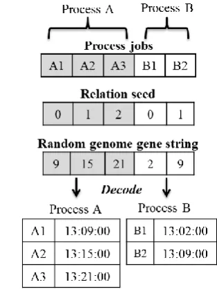
During the generation of the initial population of candidate solutions, to ensure that all genomes comply with this rule and to ensure job order is maintained, the string of genes representing the individual jobs are grouped according to their parent process and job order. A relation seed of equal length to the gene string is then generated based on job order. This consists of a number which increments with every gene and resets back to zero when a process ends. An example of a two process gene string can be seen in Fig. 1. In this example, the relation seed is used by the random number generator to ensure the random numbers comply with the job order.

Let R = {r0, …, rN-1} denote the relation seed with N

denoting the total number of jobs, S = {s0, …, sN-1} the job

start time, G = {g0, …, gN-1} the genome representation of S,

and D = {d1, …, dL} the process deadline time with L

denoting the total number of processes. To reduce the computation time and to increase the probability of generating a valid schedule, the search of optimum G is

concentrated in a smaller sub-space by limiting the range of random time generation for each job start. If a job is denoted by i and belongs to a process denoted by u with deadline du,

then the candidate job start time represented is given by

{

} (1)

This ensures that, within a process group, the next randomly generated gene (job start time) will be larger than the previous. It also permits the jobs belonging to different processes to potentially run concurrently as demonstrated in Fig. 1 by jobs A1 and B2 starting at the same time.

Fig. 1. Example of a relation seed generated based on job order and parent process order. In this example, T = 00:01:00 and se= 13:00:00.

In order to convert between genome representation G and a list of job start times S, an encoding / decoding function is used. In the original schedule, the earliest start time se is

used as a reference point for encoding and decoding job start time si to or from gene gi.

Encoding:





T s s

g i e

i



 (2)

Decoding:





s

si  e i (3)

where T is the minimal time shift that can be applied to the job start times.

B. Algorithm Overview

To ensure the algorithm finds a solution as close to the global optimum as possible, there are two separate loops as can be seen in Fig 2. The inner loop is used to simulate multiple generations of a population within the genetic algorithm. The outer loopis used to repeat the entire genetic algorithm process a predefined number of times. For every iteration of the outer loop, a population P of Np genomes is

reproducing. In tournament selection, a subset of the main population is randomly selected and the fittest genome in that subset is placed in an interim population. This is repeated until the interim population is the same size as the original population. Tournament selection was chosen due to its implementation simplicity, which directly affects computational time. Additionally the selection diversity can be easily altered by adjusting the subset population size. Uniform crossover and mutation is then applied to the interim population. To ensure job order is maintained during crossover, if a gene is smaller than the one before it, and they are of the same parent process, its value will be modified according to (4),





 _{i i}

i g C

g (4)

where Ci-1 is the makespan of the job whose start time is

represented by gi-1.

Fig. 2. Flowchart of the genetic algorithm schedule optimiser.

Different rates of crossover probability were investigated to determine the effect on the final outcome. This is discussed further in section three. Mutation probability remains fixed at 2%. Once crossover and mutation have been applied the fitness is recalculated. The algorithm will then return up to elitism with the newly generated population until the inner loop is completed. As elitism is used, the two fittest genomes are copied and their clones bypass the crossover and mutation process. This ensures that

if the optimal value is generated in an early iteration, their clone will survive unchanged until the end while the original will reproduce to see if a fitter solution can be generated.

Once the inner loop is completed, the fittest genome generated is added to a list of fittest genomes. The outer loop then iterates and a new population is generated. This consists of Np – 1 random genomes generated using the

relation seed, and a copy of the best genome from the list of fittest genomes. For the very first iteration, the fittest genome is considered to be a direct encoding of the original schedule. All this is done for several reasons: a) the original schedule may produce the optimal energy variance already or may contain optimal components which could be extracted during crossover; b) the optimal genome from a previous iteration may be further optimised; and c) it ensures that a valid genome is always returned from the inner loop.

The entire system is not designed to stop once a particular fitness has been reached. The fitness itself is the predicted energy consumption variance, constructed from the job start times proposed in the genomes gene string and the job energy models. As the minimal variance for a manufacturing schedule cannot be known beforehand, the system is allowed to run for 1000 outer loop iterations. At this point it returns the global fittest genome. The configuration used in these experiments consists of 100 iterations of the inner loop and 1000 iterations of the outer loop. During testing it was found that as the number of jobs increased, the number of outer loop iterations also had to be raised in order to increase the likelihood of a genome fitter than the original being generated. This is due, in part, to the conditions a genome must meet to be classified as a valid schedule.

C. Fitness function

The fitness function serves two purposes: a) determine if genome G represents a valid schedule that can be executed on the proposed manufacturing line, and if it is valid, b) to decode the gene string, build a predicted energy consumption profile, and calculate the variance. The validity conditions for each genome are as follows:

For a set of job start time genes gi with a makespan of Ci, belonging to the same parent process:





 i i

i g C

g (5)

For each job with a parent process deadline dj:





j g C

d   (6)

At any time t, usage on a machine of type Mk, Mk,Usage with a maximum availability of Mk,X:

X k Usage

k t M

M _, () _, (7)

the total amount of that machine. If a particular genome fails any of these conditions it is classified as invalid and is assigned the maximum fitness, in practice this is the maximum value of a double precision number in C#. In this implementation the fittest genome is defined as the one with the minimum fitness value, and therefore minimum energy consumption variance. If a genome meets all conditions, the energy consumption variance for that schedule is calculated by generating a predicted energy consumption profile.

Initially an energy consumption profile is created for each machine m in the production line, Em. This spans from se to DMax with time spacing T and is initially populated with the

idling value for that particular machine mIdle. Then in

chronological order, for every job j using that machine jm,

their associated job specific energy consumption profile,

jProfile is copied to Em, beginning at the start time denoted by

the appropriate gene jg. This process overwrites the values

currently assigned to the associated elements of the profile. Additionally the recorded idling consumption from that particular job jIdleis subsequently assigned to the remainder

of the profile. This is because the idling energy consumption could have changed if the machine is now in a different position or configuration due to the previous job. This process is repeated until the energy profiles of all jobs running on that machine have been merged. The process described above is detailed in pseudo-code below.

Input: List of jobs each with a representative gene

specifying its start time gi. The energy consumption profiles

and idling energy consumptions for each job jProfileand jIdle.

A list of machines and their standard idling energy consumptions, M



Output: Energy profile for machine Em.

For each machine m

EM(se) to (DMax)= M,Idle

For every job j which uses m, in chronological order.

Copy jProfile to Em, beginning at gi. Copy jIdle to Em from (gi + Ci) to DMax

End End

The system assumes that when not in operation, each machine is left idling. Once the predicted energy consumption profile is generated for each machine, the total predicted energy consumption profile for a total of X machines can be calculated using (8).



 X

m m

Total t E t

E

1 ( )

)

( (8)

From (8), the variance of the predicted total energy consumption profile is given by:









 Max

e D

s

t Total Total

e Max

Var E E

S D

T

E (9)

where DMax = max{d1,…, L} and ETotaldenotes the average energy consumption. Once calculated the sample variance is assigned as the genomes fitness value.

III. EXPERIMENTS AND RESULTS

The proposed genetic algorithm was tested with multiple simulated schedules of increasing complexity. These schedules were devised based on real schedules and their job specific energy consumption profiles incorporate waveform characteristics such as inrush currents and transients. Each schedule file contains details of the processes and jobs, the energy profiles for each job, and the idling power consumptions for each machine. A separate file contains data related to the specification of the individual manufacturing lines.

In the first set of experiments, the performance of the proposed genetic algorithm was evaluated by modifying low complexity schedules and comparing against the calculated actual optimal result. This actual optimal result was determined by generating all possible combinations of time steps and selecting the one which produced the lowest energy consumption variance. For N jobs to be completed by DMax, the number of possible gene combinations is

Among the first set of experiments, a schedule containing five jobs with a maximum deadlines of 25 time steps was the most complex schedule considered, where every possible combination was generated with the corresponding energy consumption profile. This proved that the algorithm was successful in finding the optimum solution among 255 = 9,765,635 possible solutions.

In the first set of experiments, different values for crossover probability and tournament selection size were also investigated to determine the optimal values. For

PCrossover, 0.65, 0.75, and 0.85 were selected. This range was

chosen as a probability any higher than 85% would cause too much disruption to a population. This may result in a possible optimal solution being lost before it can be identified. This has been concluded by other authors [15]. A value less than 65% would not allow a population to sufficiently reproduce. For NTournament values, Np/8, Np/6and Np/4 were investigated. Each combination was tested ten

times to determine the number of iterations required to return a near optimal solution.

The number of iterations presented in table I demonstrate that the algorithm works most efficiently at low rates of crossover probability with a high tournament selection size. All results produced in the second set of experiments are generated with the algorithm set to these parameters.

Table I

Average number of iterations until optimal value generated with differing crossover rate and tournament selection size.

PCrossover

0.65 0.75 0.85

NTournament

Np/8 161.875 128.5 165

Np/6 203.25 218.375 242

Np/4 101.625 123 186.625

In the second set of experiments, the proposed genetic algorithm was applied to more complex schedules with N > 5. The experiments show that with schedules with a large amount of downtime, the optimal solution appears to be generated quicker. This is likely due to the fact that while more downtime increases DMax, it also increases the

probability of a proposed schedule being valid in accordance with fitness function condition (6). Additionally, the optimal solution generated by repeatedly running the algorithm ten times with the same schedule is not concise. This is to be expected as genetic algorithms may not find the most optimal solution in the time allotted to them. However the optimal results produced by each only vary slightly. With only a small range of returned values, it can be assumed that the proposed schedule that produced it is a near optimal solution.

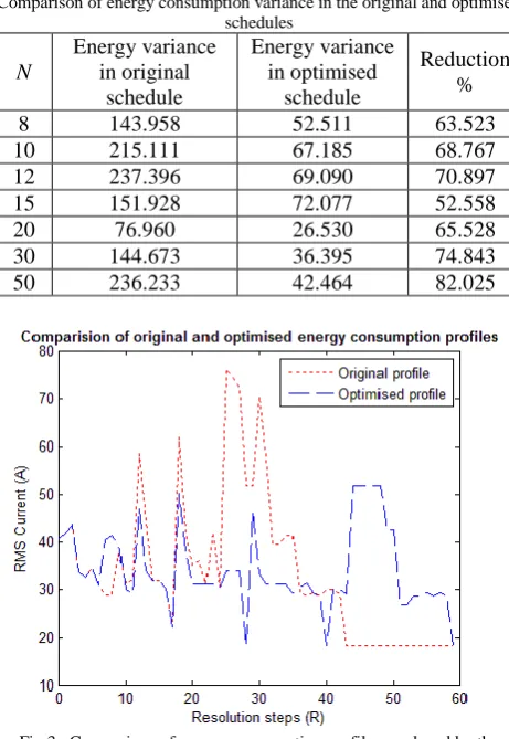
Table II

Comparison of energy consumption variance in the original and optimised schedules

N

Energy variance in original

schedule

Energy variance in optimised

schedule

Reduction %

8 143.958 52.511 63.523

10 215.111 67.185 68.767

12 237.396 69.090 70.897

15 151.928 72.077 52.558

20 76.960 26.530 65.528

30 144.673 36.395 74.843

50 236.233 42.464 82.025

Fig 3. Comparison of energy consumption profiles produced by the original and optimised schedules. Ns= 12. Original variance = 237.396,

optimised variance = 69.09

Table II demonstrates the reduction in variance that can be achieved, compared to the original energy consumption variance. Fig. 3 shows the effect on the energy consumption profile as an example. It can be seen in Fig. 3 that by redistributing the jobs the energy consumption profile can alter significantly. This can potentially result in a large percentage reduction in the overall variance. However this level of reduction will be dependent on the optimisation of the original schedule, the available downtime, and the individual job specific energy consumption profiles. If for example, a schedule consists of jobs whose energy consumption changes very little over time, and there is very little downtime before the deadline, it may not be possible to optimise this schedule significantly.

IV. CONCLUSION

This paper presents a methodology for modifying a manufacturing production schedule with a goal to minimise the variance in the production line energy consumption. The use of a genetic algorithm for individual job start time manipulation is detailed and the algorithms internal parameters are evaluated and optimised based on experimental data. For a series of scheduled processes, the algorithm is found to be successful in reducing the energy consumption variance to its near minimum, while ensuring that manufacturing resource limitations and process deadlines are never exceeded. While the global optimum solution is not guaranteed to be returned, a solution near the global optimum is always produced. For each potential solution, a predicted energy consumption profile is generated based on job specific energy models. The variance of the predicted energy profile is then calculated. At the end of the algorithm, the solution which holds the minimal variance is concluded to be the most optimal. However the accuracy of the system is entirely dependent on the accuracy and resolution of the energy models and the minimal time shift that can be applied to each job, T. For the work presented in this paper, mock energy models based on real job consumption profiles were utilised. For real implementations, it is recommended that the resolution of the models be significantly higher than T. However, with suitably accurate models a significant reduction in energy consumption variance can be achieved regardless of the amount of jobs in the schedule. Through empirical testing an average reduction percentage of approximately 70% has been achieved. It is also seen that the reduction percentage is independent of the schedule job count with a range between 8 to 50 jobs tested.

If the methodologies described in this paper were implemented in a real manufacturing production line with struggling power distribution capabilities, the reduced variance could potentially allow for another process, with a suitable optimised energy consumption variance, to run without needing to reinforce the local infrastructure. These methodologies could also allow a manufacturing production line to be power entirely from limited supply resources, such as renewable energy sources.

ACKNOWLEDGEMENT

The authors would like to thank the industrial supervisors Damian Adams and Stuart Barker of BAE Systems (Operations) Ltd. There insights and dedication has proven invaluable to the success of this work.

REFERENCES

[1] D. Karger, C. Stein, J. Wein, “Scheduling Algorithms,” Algorithms and Theory of Computation Handbook, 2nd ed. Florida, USA: Chapman & Hall/CRC, 2009, pp 20-1 – 20-34.

[2] K. Fang, N. Uhan, F. Zhao, J.W. Sutherland, “Flow Shop Scheduling with Peak Power Consumption Constraints,” Annals of Operations Research, vol. 206, issue 1, pp 115 – 145, Jul. 2013

[4] K. Fang, N. Uhan, F. Zhao, J.W. Sutherland, “A New Shop Scheduling Approach in support of Sustainable Manufacturing,” Glocalized Solutions for Sustainability in Manufacturing, pp 305 – 310, May 2011

[5] Transfact. Energy in Production Planning and Scheduling (E-PPS) [Online]. Available: http://www.transfact.de/EN/

[6] Department of Energy & Climate Change, “Energy Consumption in the UK – Industrial Factsheet,” ch. 4, pp 3 [Online]. Jul. 2013 Available: https://www.gov.uk/

[7] G. Mouzon, M.B. Yildirim, J. Twomey, “Operational Methods for Minimization of Energy Consumption of Manufacturing Equipment,” International Journal of Production Research, vol. 45, issue 18-19, Dec 2010

[8] P. Eberspächera, A. Verla, “Realizing Energy Reduction of Machine Tools Through a Control-integrated Consumption Graph-based Optimization Method,” Forty Sixth CIRP Conference on Manufacturing Systems 2013, vol. 7, pp 640 – 645, 2013

[9] G.D. Orio, G. Candido, J. Barata, J.L. Bittencourt, R. Bonefeld, “Energy Efficiency in Machine Tools – A Self-Learning Approach,” 2013 IEEE International Conference on Systems, Man, and Cybernetics, pp 4878 – 4883, Oct 2013

[10] M.B. Yildirim, G. Mouzon, “Single-Machine Sustainable Production Planning to Minimize Total Energy Consumption and Total Completion Time Using a Multiple Objective Genetic Algorithm,” IEEE Transactions on Engineering Management, vol. 59, issue 4, pp. 585 – 597, Nov. 2012

[11] S. Yassa, J. Sublime, R. Chelouah, H. Kadima, G. -S. Jo, B. Granado, “A Genetic Algorithm for Multi-Objective Optimisation in Workflow Scheduling with Hard Constraints,” International Journal of Metaheuristics, vol. 2, no. 4, pp. 415 – 433, 2013

[12] J.F. Gonçalves, J.J.M. Mendes, M.G.C. Resende, “A Genetic Algorithm for the Resource Constrained Multi-Project Scheduling Problem,” European Journal of Operational Research, vol. 189, issue 3, pp 1171 – 1190, Sep. 2008

[13] N. Brown, R. Greenough, K. Vikhorev, S. Khattak, “Precursors to using Energy Data as a Manufacturing Process Variable,” 6th _IEEE

International Conference on Digital Ecosystems Technologies, pp 1 – 6, Jun. 2012

[14] F. Herrera, M. Lozano, J.L. Verdegay, “Tackling Real-Coded Genetic Algorithms: Operators and Tools for Behavioural Analysis,” Artificial Intelligence Review, vol. 12, issue 4, pp. 265 – 319, Aug. 1998